PROJECT 2 - RANKINE CYCLE SIMULATOR

ABSTARCT

This report is regarding MATLAB code for determining state points parameters of Rankine Cycle Simulator in relation to user inputs and additionally plotting T-S and H-S plots. The theory about Rankine cycle simulator working is explained and finally Net work output, work ratio and the thermal efficiency are also calculated. The step-by-step code generation in MATLAB and logic is explained and errors appeared during process of successful execution of code and steps are taken to resolve them. Additionally, evidence of errors is documented in the report.

THEORY

The following paragraphs gives a brief account on thermodynamics and Rankine Cycle working.

THERMODYNAMICS

It is science of the relationship between heat, work, temperature, and energy. In wide sense, it deals with the transfer of energy from one point to another and from one form to another form. The crucial concept is that heat is a form of energy corresponding to a definite amount of mechanical work. Thermodynamics is the study of the effects of work, heat, and energy on a system. Thermodynamics is only concerned with macroscopic (large-scale) changes and observations.

In thermodynamics, the following are predominantly used technical terms for better understanding.

1. System: it is prescribed region of space or finite quantity of matter nearby an envelope/casing called the boundary.

the following are three types of system:

1. Closed System: there is no mass transfer, but heat transfer takes place with surroundings and system.
2. Open System: there is mass transfer and heat transfer between surroundings and system.
3. Isolated System: there is no mass transfer and no heat transfer between surroundings and system.
4. Surrounding: the space and matter external to the thermodynamic system and outside boundary is called the surrounding.
5. Universe: it is combination of system and the surroundings put together are called universe.
6. State: the distinctive circumstance of the system at particular point of time and described by properties.
7. Process: the line(path) of series or succession of points through which the system passes during transformation from one state to another state is called process.
8. Cycle: the process of going through various states and returning to initial state of system is called cycle.

All of thermodynamics can be expressed in terms the following:

-Temperature (T)

-Internal Energy (U)

-Entropy (S)

-Heat (Q)

-Work(W)

THERMODYNAMICS PROCESS FOR CLOSED SYSTEM

The following are the thermodynamic process:

1. Isothermal process: it is a constant temperature process. The heat flow into or out of the system must be slow enough to maintain thermal equilibrium. The energy entering system must leave with work.

For ideal gases, if ΔT is zero, ΔU = 0

Therefore, Q = W

2. Isobaric Process: is a constant pressure process. ΔU, W, and Q are generally non-zero, but calculating the work done by an ideal gas is straightforward.

W = P·ΔV

3. Isochoric Process: is a constant volume process. When the volume of a system doesn’t change, it will do no work on its surroundings. W = 0. Heating gas in a closed container is an isochoric process

ΔU = Q

4. Polytropic Process: is a thermodynamic process that obeys the relation: where p is the pressure, V is volume, n is the polytropic index, and C is a constant. The polytropic process equation can describe multiple expansion and compression processes which include heat transfer. The exponent nis known as the polytropic index and it may take on any value from 0 to ∞, depending on the particular process.

pVⁿ = constant

5. Adiabatic Process: it is the process in which there is no exchange of heat from the system to its surrounding neither during expansion nor during compression. It can be either reversible or irreversible. Following are the essential conditions for the adiabatic process to take place: First, the system must be perfectly insulated from the surrounding. Second, the process must be carried out quickly so that there is a sufficient amount of time for heat transfer to take place.

PV^γ = constant

P is the pressure of the system

V is the volume of the system

γ is the adiabatic index and is defined as the ratio of heat capacity at constant pressure C_p to heat capacity at constant volume C_v.

6. Isentropic Process: An isentropic process is a thermodynamic process, in which the entropy of the fluid or gas remains constant. It is a special case of an adiabatic process in which there is no transfer of heat or matter. It is a reversible adiabatic process. An isentropic process can also be called a constant entropy process. In engineering such an idealized process is very useful for comparison with real processes.

Since there is change in internal energy (dU) and changes in system volume (∆V), so, the entahlpy of the system, which is defined as:

H = U + pV

dH = dQ + Vdp

dH = TdS + Vdp

THERMODYNAMICS LAWS:

The following are the laws of thermodynamics which used to determine heat, work, energy, enthalpy and entropy.

1.Zeroth Law of Thermodynamics: If two systems are separately in thermal equilibrium with a third system, they are in thermal equilibrium with each other.

2.First Law of Thermodynamics: In cyclic process the cyclic integral of the heat transfer to the system is equal to the cyclic integral of the work transfer to the surroundings. The internal energy of an isolated system is constant. A closed system may exchange energy as heat or work. Let us consider a close system at rest without external fields.

The first law of thermodynamics is actually the law of conservation of energy stated in a form most useful in thermodynamics. The first law gives the relationship between heat transfer, work done, and the change in internal energy of a system. The First Law is often called the conservation of energy law.

Mathematically stated, for a control mass undergoing a cyclic process such as in Joule’s experiment and for consistent set of units

∫dQ_{from system}= ∫dW_{on system}

or ∫dQ_{from system}- ∫dW_{on system} = 0

The important thing to remember is that the first law states that the energy is conserved always.

Sign convention , the work done by a system on the surroundings is treated as a positive quantity. Likewise, energy transfer as heat to the system from the surroundings is assigned a positive sign. With the sign convention one can write:∫dQ = ∫dW

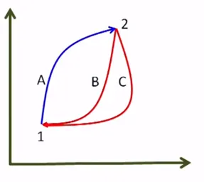
Consequences of the first law: Suppose a system is taken from state 1 to state 2 by the path 1-a-2 and is restored to the initial state by the path 2-b-1, then the system has undergone a cyclic process 1-a-2-b-1. If the system is restored to the initial state by path 2-c-1, then the system has undergone the cyclic change 1-a-2-c-1. Let us apply the first law of thermodynamics to the cyclic processes 1-a-2-b-1 and 1-a-2-c-1 to obtain

∫_1-a-2dQ+ ∫_2-b-1dQ - ∫_1-a-2dW - ∫_2-b-1dW =0

∫_1-a-2dQ+ ∫_2-c-1dQ - ∫_1-a-2dW - ∫_2-c-1dW=0

Subtracting, we get

∫_2b1dQ- ∫_2c1dQ –( ∫_2b1dW - ∫_2c1dW) =0

We know that the work is a path function and hence the term in the bracket is non-zero. Hence, we find

∫_2b1dQ = ∫_2c1dQ

That is heat is also a path function.

Energy is a property of the system: By rearranging we can have

∫_2b1 (dQ - dW) = ∫_2c1 (dQ - dW)

It shows that the integral is the same for the paths 2-b-1 and 2-c-1, connecting the states 2 and 1. That is, the quantity ∫ (dQ - dW) does not depend on the path followed by a system, but depends only on the initial and the final states of the system. That is ∫ (dQ - dW) is an exact differential of a property. This property is called energy (E). It is given by

dE = dQ-dW

E = KE + PE +U

where U is the internal energy. Therefore,

dE = d(KE) + d(PE) + dU = dQ-dW

Quit often in many situations the KE or PE changes are negligible.

dU = dQ – dW

An isolated system does not exchange energy with the surroundings in the form of work as well as heat. Hence dQ = 0 and dW = 0. Then the first law of thermodynamics reduces to dE = 0 or E₂ = E₁ that is energy of an isolated system remains constant.

3.Second Law of Thermodynamics: it introduces the notion of entropy (S), a measure of system disorder. It is about the quality of energy. It states that as energy is transferred or transformed, more and more of it is wasted. The Second Law also states that there is a natural tendency of any isolated system to degenerate into a more disordered state.

This law is also described two scientist statement:

KELVIN-PLANK STATEMNT: it is impossible to construct a device that will operate in cycle and produces no effect other than the rising of a weight and the exchange of heat with a single reservoir.

CLAUSIUS STATEMNT: It is impossible to construct a device that operates in a cycle and produce no effect other than the transfer of heat from cooler body to hotter body.

4. Third Law of Thermodynamics: It is impossible to reach a temperature of absolute zero. This is another statement of third law, the entropy of a true equilibrium state of a system at T = 0 K is zero. Strictly speaking, this is true only if the quantum mechanical ground state is non-degenerate. If it is degenerate, the entropy at T = 0 K is a small constant, not 0!)

Absolute entropy can be written as S=kBlogW, where

W is the number of available microstates

k_B is the Bolzmann constant

Provided that the ground state is unique (or W=1), the entropy of a perfect crystal lattice as defined by Nernst’s theorem is zero provided that its ground state is unique, because log(1) =0.

The third law of thermodynamics is sometimes stated as follows: The entropy of a perfect crystal at absolute zero is exactly equal to zero.

At zero kelvin the system must be in a state with the minimum possible energy, thus this statement of the third law holds true if the perfect crystal has only one minimum energy state. Entropy is related to the number of possible microstates, and with only one microstate available at zero kelvin the entropy is exactly zero.

Principles of thermodynamics are useful for power cycle for of electric power generation (i.e net power output) and to study refrigeration & heat pump which requires input of net power.
Classification of thermodynamics power cycles can be done into two types:

1. Vapor cycle working fluid exists in liquid phase during one part of the cycle (i.e from condenser outlet to Boiler) and mixed phase wit in the steam boiler and in vapor phase at the Boiler outlet.
2. Gas cycle working fluid during the cycle remains in gas phase.

Steam power generation units run on vapor power cycle using water as the working fluid.
Under this section attempt is made to familiarize the readers with the concepts of ideal vapor cycle called Rankine cycle.

Entropy: it is the measure of a system's thermal energy per unit temperature that is unavailable for doing useful work. Because work is obtained from ordered molecular motion, the amount of entropy is also a measure of the molecular disorder, or randomness, of a system.

Enthalpy: it is a concept used in science and engineering when heat and work need to be calculated. When a substance changes at constant pressure, enthalpy tells how much heat and work was added or removed from the substance. Enthalpy is similar to energy, but not the same. Enthalpy, the sum of the internal energy and the product of the pressure and volume of a thermodynamic system. In symbols, the enthalpy, H, equals the sum of the internal energy, E, and the product of the pressure, P, and volume, V, of the system: H = E + PV.

RANKINE CYCLE: It is the basic operating cycle for all power plants where a working fluid is continuously changing its phase from liquid to vapor and vice-versa. It is well known as modified Carnot cycle , where condensation process is continued until the steam condensed in to water.

Rankine cycle is also defined: if the working fluid in a vapor cycle passes through various components of the power plant without irreversibility and frictional pressure drop, then the cycle is called as Ideal Rankine Cycle.

Many of the impracticalities associated with the Carnot cycle can be eliminated by superheating the steam in the boiler and condensing it completely in the condenser. The cycle that results is the Rankine cycle, which is the ideal cycle for vapor power plants. The ideal Rankine cycle does not involve any internal irreversibility. The below picture depicts Rankine cycle.

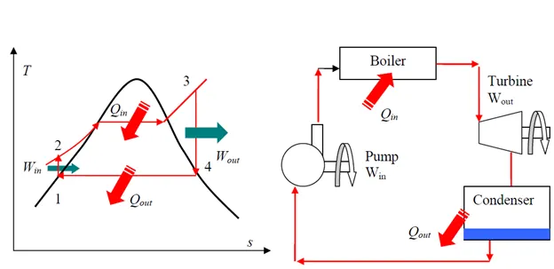
PROCESS_1-2 ISENTROPIC COMPRESSION: Water enters the pump as state 1 as saturated liquid and is compressed isentropically to the operating pressure of the boiler.

PROCESS_2-3 CONST PRESSURE HEAT ADDITION: Saturated water enters the boiler and leaves it as superheated vapor at state 3.

PROCESS_3-4 ISENTROPIC EXPANSION: Superheated vapor expands isentropically in turbine and produces work.

PROCESS_4-1 CONST PRESSURE HEAT REJECTION: High quality steam is condensed in the condenser.

Energy Analysis of the Ideal Rankine Cycle: All four components of the Rankine cycle are steady-state steady-flow devices. The potential and kinetic energy effects can be neglected. The first law per unit mass of steam can be written as:

steady-flow energy equation:

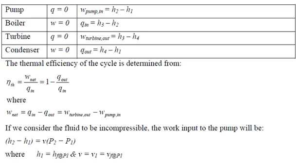
The thermal efficiency can be interpreted as the ratio of the area enclosed by the cycle on a T-s diagram to the area under the heat-addition process.

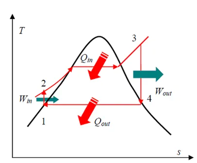
Deviation of actual vapor power cycles from idealized one: The actual vapor power cycle differs from the ideal Rankine cycle as a result of irreversibility in various components. Fluid friction and heat loss to the surroundings are the two common sources.

The below picture depicts the deviation:

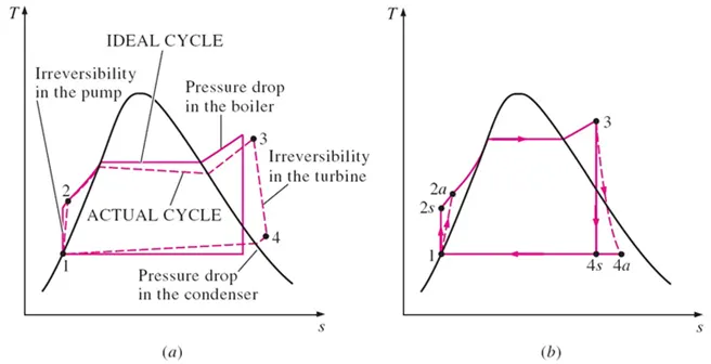
Based on the variation the thermal efficiency of pump and turbine changes. The below are formulas.

INCREASE THE EFFICIENCY OF THE RANKINE CYCLE: the following are methods to enhance efficiency. The basic idea behind all the modifications to increase the thermal efficiency of a power cycle is the same: Increase the average temperature at which heat is transferred to the working fluid in the boiler, or decrease the average temperature at which heat is rejected from the working fluid in the condenser.

Lowering the Condenser Pressure (Lowers T__{low, avg}): To take advantage of the increased efficiencies at low pressures, the condensers of steam power plants usually operate well below the atmospheric pressure. There is a lower limit to this pressure depending on the temperature of the cooling medium.

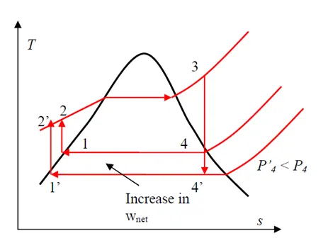
Side effect: Lowering the condenser pressure increases the moisture content of the steam at the final stages of the turbine.

Superheating the Steam to High Temperatures (Increases T_high,avg)

Both the net work and heat input increase as a result of superheating the steam to a higher temperature. The overall effect is an increase in thermal efficiency since the average temperature at which heat is added increases. Superheating to higher temperatures decreases the moisture content of the steam at the turbine exit, which is desirable. The temperature is limited by metallurgical considerations. Presently the highest steam temperature allowed at the turbine inlet is about 620°C.

Increasing the Boiler Pressure

For a fixed turbine inlet temperature, the cycle shifts to the left and the moisture content of steam at the turbine exit increases. This side effect can be corrected by reheating the steam. Increasing the operating pressure of the boiler leads to an increase in the temperature at which heat is transferred to the steam and thus raises the efficiency of the cycle. The below is the picture depicts.

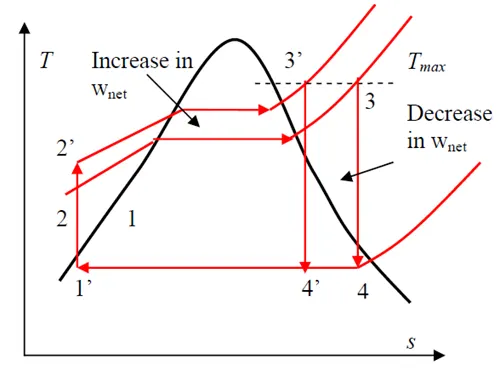
Note that for a fixed turbine inlet temperature, the cycle shifts to the left and the moisture content of the steam at the turbine exit increases. This undesirable side effect can be corrected by reheating the steam.

The Ideal Reheat Rankine Cycle

To take advantage of the increased efficiencies at higher boiler pressure without facing the excessive moisture at the final stages of the turbine, reheating is used. In the ideal reheating cycle, the expansion process takes place in two stages, that is the high-pressure and low-pressure turbines.

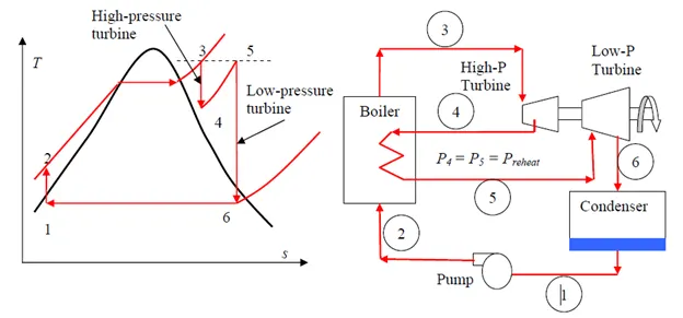
The total heat input and total turbine work output for a reheat cycle become:

The incorporation of the single reheat in a modern power plant improves the cycle efficiency by 4 to 5 percent by increasing the average temperature at which heat is transferred to the steam.

The Ideal Regenerative Rankine Cycle

The regeneration process in steam power plants is accomplished by extracting (or bleeding) steam from turbine at various stages and feed that steam in heat exchanger where the feedwater is heated. These heat exchangers are called regenerator or feedwater heater (FWH). FWH also help removing the air that leaks in at the condenser (de-aerating the feedwater). There are two types of FWH’s, open and closed.

Open (Direct‐Contact) Feedwater Heaters

An open FWH is basically a mixing chamber where the steam extracted from the turbine mixes with the feedwater exiting the pump. Ideally, the mixture leaves the heater as a saturated liquid at the heater pressure. The following are the features of the OFWH:

- Simple

- inexpensive

- good heat transfer characteristics

- bring feedwater to the saturation state

- a pump is required for each FWH

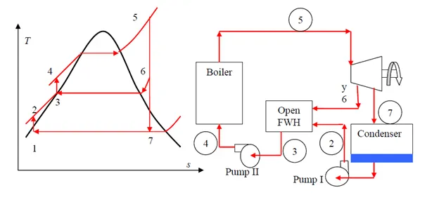
Based on above figure, the heat and work interactions of a regenerative Rankine cycle with one FWH can be expressed per unit mass of steam flowing through the boiler as:

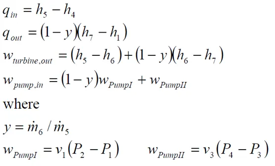
Thermal efficiency of the Rankine cycle increases as a result of regeneration since FWH raises the average temperature of the water before it enters the boiler. Many large power plants have as many as 8 FWH’s.

Closed Feedwater Heaters

In closed FWH, heat is transferred from the extracted steam to the feedwater without any mixing taking place. Thus; two streams can be at different pressures, since they don’t mix. In an ideal closed FWH, the feedwater is heated to the exit temperature of the extracted steam, which ideally leaves the heater as a saturated liquid at the extraction pressure. The below T-S diagram depicts it.

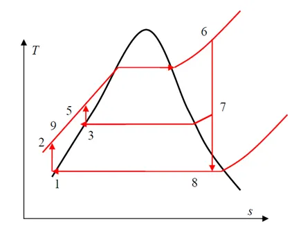
The below is the picture that depicts Ideal regenerative Rankine cycle with a closed FWH.

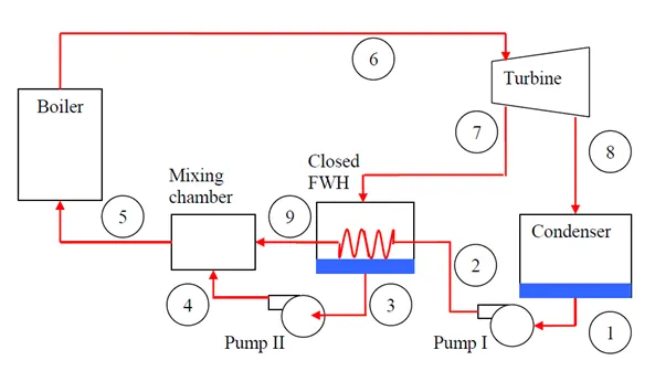
The following features of Closed FWH:

- More complex (internal tubing)

- less effective (no mixing)

- do not require a pump for each FWH

The "dryness fraction", x, gives the fraction by mass of gaseous water in the wet region, the remainder being droplets of liquid.

The ratio of the compressor work to the turbine work is called the back-work ratio. Sometimes, more than one-half of the turbine work may be used by the compressor.

UNITS

The following are units of the parameters involved:

T- Temperature °C

p -Pressure bar

h- Enthalpy kJ/kg

v -Specific volume m3/kg

rho -Density kg/ m3

s -Specific entropy kJ/(kg °C)

u- Specific internal energy kJ/kg

Cp -Specific isobaric heat capacity kJ/(kg °C)

Cv- Specific isochoric heat capacity kJ/(kg °C)

work done by turbine- KJ/Kg

work done on pump- KJ/Kg

net work done- KJ/Kg

specific heat consumption- Kg/kWh

MATLAB CODE STEP-BY-STEP DESCRIPTION

The following are various steps involved in generating code to determine the various parameters for Rankine cycle efficiency. Initially, MATLAB code ask user to input his choice to calculate efficiency of Rankine cycle or not, then MATLAB code takes inputs from the user to determine parameters at various states in the Rankine cycle, further, the code will calculate work done on pump, turbine work, net work, heat input for heating condensed water and finally thermal efficiency and specific heat consumption. The following are steps involved:

1.Starting code with comment box to inform about what is purpose MATLAB code and using ‘close all‘, ‘clear all’, ‘clc’ functions. The 'clear all': this function removes all variables, functions and MEX-files from-memory and leaving workspace empty. The 'close all': This function will close all the figure handles are visible and hidden figure handles. The 'clc': function clears text from function window.

close all

clear all

clc

2. I used ‘while’ loop to ask the user to provide his choice of interest to calculate the parameters of Rankine cycle.

while(1)

3. I used 'cprintf.m' function to show all the process of Rankine Cycle Simulator in color font. The below is the code

cprintf('Blue','\n RANKINE CYCLE SIMULATION \n\n')

cprintf('Red','1-2 ISENTROPIC EXPANSION IN THE TURBINE \n')

cprintf('Magenta','2-3 CONSTANT PRESSURE HEAT REJECTION BY THE CONDENSOR \n')

cprintf('Red','3-2 ISENTROPIC COMPRESSION IN THE PUMP \n')

cprintf('Magenta','4-1 CONSTANT PRESSURE HEAT ADDITION BY THE BOILER \n')

4. Here, I asked user opinion of calculating Rankine cycle efficiency or not based on his choice, I used ‘if-else’ function to proceed further. User input is important.

I_P=input('\n DO YOU WANT TO CALCULATE RANKINE CYCLE DETAILS ? Y or y/N or n:','s');

I_P_U=upper(I_P);

When user presses ‘y’ or ‘Y’, the MATLAB will proceed to execute the code to calculate parameters.

if I_P_U=='Y'

5. Now, I used the ‘close’ function to close all the figure window plots, there are any so that I could plot new plots for Temperature Vs Entropy and Enthalpy Vs Entropy plots based on user input parameters.

close(figure(1),'reset')

close(figure(2),'reset')

6. Now, I used the ‘input’ function for providing user input for turbine inlet pressure, temperature and input to the condenser pressure of the steam or combination of liquid and vapor.

PRESS_1=input(' ENTER THE TURBINE INLET PRESSURE (in bar): ');

TEMP_1=input('\n ENTER THE TURBINE INLET TEMPERATURE (in Degree Celsius): ');

PRESS_2=input('\n ENTER THE INSIDE CONDENSOR PRESSURE (in bar): ');

7. I used ‘Xsteam.m’ function file which consist of certain parameters required for the calculations. Steam and water properties for MATLAB based on the "International Association for Properties of Water and Steam Industrial Formulation 1997 (IAPWS IF-97). A full implementation of the IF-97 standard that provides very accurate steam and water properties in ranges from 0-1000 bar and 0-2000°C. Provided thermodynamic properties are:

Temperature
Pressure
Enthalpy
Specific volume
Density
Specific entropy
Specific internal energy
Specific isobaric heat capacity
Specific isochoric heat capacity
Speed of sound
Viscosity
Vapor fraction

All properties can be calculated with the inputs, p and T known, p and h known, h and s known and some with pressure and density known. X Steam are a full implementation of the IF-97 formulation including all regions and all backward functions for good calculation speed. The code is speed optimized with pressure and enthalpy as inputs for dynamic simulations.

Now, I extracted specific heat for liquid and vapor states for given pressures at state 1 and state 2.

SPEC_HEAT_1_LIQUID=XSteam('CpL_p',PRESS_1);

SPEC_HEAT_1_VAPOUR=XSteam('CpV_p',PRESS_1);

SPEC_HEAT_2_LIQUID=XSteam('CpL_p',PRESS_2);

SPEC_HEAT_2_VAPOUR=XSteam('CpV_p',PRESS_2);

Where

CpV_p -saturated vapor heat capacity

CpL_p -saturated liquid heat capacity

8. Correspondingly, I used the ‘XSteam.m’ function to extract saturation temperature for given pressures at state1 and state 2.

SAT_TEMP_P1=XSteam('Tsat_p',PRESS_1);

SAT_TEMP_P2=XSteam('Tsat_p',PRESS_2);

Where, Tsat_p -saturation temperature at given pressure

At the same time, I am verifying the input temperature is greater or equal to saturation temperature for given pressure at state 1, for that I used ‘if-else’ function.

if not (TEMP_1>=SAT_TEMP_P1)

cprintf('_red','You entered Inlet Temperature less than Saturation Temperature\n')

cprintf('_blue','\n Please enter the Inlet Temperature greater or equal to Saturation Temperature\n')

else

9. Once, above condition passed, then, I am using ‘XSteam.m’ function for extracting all the saturated entropy, enthalpy for both liquid and vapor phases for all the state points .

Saturation properties at state1

ENTHALPY_VAP_STATE_1=XSteam('hV_p',PRESS_1);

ENTROPY_VAP_STATE_1=XSteam('sV_p',PRESS_1);

ENTHALPY_LIQ_STATE_1=XSteam('hL_p',PRESS_1);

ENTROPY_LIQ_STATE_1=XSteam('sL_p',PRESS_1);

Saturation properties at state2

ENTHALPY_VAP_STATE_2=XSteam('hV_p',PRESS_2);

ENTROPY_VAP_STATE_2=XSteam('sV_p',PRESS_2);

Saturation properties at state3

ENTHALPY_LIQ_STATE_3=XSteam('hL_p',PRESS_2);

ENTROPY_LIQ_STATE_3=XSteam('sL_p',PRESS_2);

Saturation properties at state4

ENTHALPY_LIQ_STATE_4=XSteam('hL_p',PRESS_1);

ENTROPY_LIQ_STATE_4=XSteam('sL_p',PRESS_1);

Uniformly, I utilized XSteam.m function to obtain entropy and enthalpy at state 1 with respect to pressure and temperature at state 1.

ENTHALPY_1=XSteam('h_pT',PRESS_1,TEMP_1);

ENTOPRY_1=XSteam('s_pT',PRESS_1,TEMP_1);

Based on Rankine cycle, constant pressure heat rejection by the condenser constant pressure heat addition, so pressure at state 4 is equal to pressure at state 1, likewise, pressure at state 3 is equal to pressure at state 2.

PRESS_4=PRESS_1;

PRESS_3=PRESS_2;

Now, I obtained enthalpy , entropy and temperature for the state 3 using XSteam.m function.

ENTHALPY_LIQ_STATE_3=XSteam('hL_p',PRESS_3);

ENTHALPY_3=ENTHALPY_LIQ_STATE_3;

ENTROPY_LIQ_STATE_3=XSteam('sL_p',PRESS_3);

ENTOPRY_3=ENTROPY_LIQ_STATE_3;

SAT_TEMP_P3=XSteam('Tsat_p',PRESS_3);

TEMP_3=SAT_TEMP_P3;

It is known fact that for isentropic expansion process the entropy at state 2 is equal to entropy at state 1.

ENTOPRY_2=ENTOPRY_1;

Between state 2 to state 3 is constant pressure heat rejection and temperature remaining same and there are entropy changes. Entropy in liquid phase and vapor phase are extracted form ‘XSteam.m’ function.

TEMP_2=TEMP_3;

ENTROPY_LIQ_STATE_2=XSteam('sL_p',PRESS_2);

ENTROPY_VAP_STATE_2=XSteam('sV_p',PRESS_2);

Now , I would be calculating dryness fraction .The steam dryness fraction is used to quantify the amount of water within steam. If steam contains 10% water by mass, it's said to be 90% dry, or have a dryness fraction of 0.9. From state 1 to state 2 is isentropic expansion process, where we get output through the turbine. Once work is obtained the power of steam get lower and it will be in the phase of both liquid and vapor, so at this point I would be calculating dryness fraction with help of entropy, entropy liquid phase and entropy vapor phase at state 2.

X2=(ENTOPRY_2-ENTROPY_LIQ_STATE_2)/(ENTROPY_VAP_STATE_2-ENTROPY_LIQ_STATE_2);

Simultaneously, I procure vapor and liquid phase of enthalpy at state2 with respect to pressure state 2 from XSteam.m function.

ENTHALPY_VAP_STATE_2=XSteam('hV_p',PRESS_2);

ENTHALPY_LIQ_STATE_2=XSteam('hL_p',PRESS_2);

Now, I determine the enthalpy at state 2, by using dryness fraction, vapor and liquid phase of enthalpy at state2.

ENTHALPY_2=ENTHALPY_LIQ_STATE_2+X2*(ENTHALPY_VAP_STATE_2-ENTHALPY_LIQ_STATE_2);

It is fact that the process of isentropic compression gives us the entropies same, the entropy at state 4 is equal to entropy at state 3.

ENTOPRY_4=ENTOPRY_3;

For determining temperature at state 4, I have to calculate Gama which is obtained specific isobaric heat capacity and specific isochoric heat capacity. The following is the code

SPEC_ISO_CHO_CAPACITY_4=XSteam('Cv_ps',PRESS_4,ENTOPRY_4);

SPEC_ISO_BAR_CAPACITY_4=XSteam('Cp_ps',PRESS_4,ENTOPRY_4);

GAMA_4=SPEC_ISO_BAR_CAPACITY_4/SPEC_ISO_CHO_CAPACITY_4;

TEMP_4=TEMP_3*((PRESS_4/PRESS_3)^((GAMA_4-1)/(GAMA_4)));

After above calculations, I convert pressure at state 3 and state 4 converted from ‘bar’ to ‘mpa’ as I calculate the work done on pump using pressure and volume at state 3.

VOLUME_3=XSteam('vL_p',PRESS_3);

WORK_PUMP=VOLUME_3*(PRESS_4_mpa-PRESS_3_mpa)*1000;

ENTHALPY_4=ENTHALPY_3-WORK_PUMP;

INLET_HEAT=ENTHALPY_1-ENTHALPY_4;

10. At this point, I determine work output produced by turbine, net work done, thermal efficiency, back work ratio and SSC(specific heat consumption). The following is the code.

TURBINE_WORK=ENTHALPY_1-ENTHALPY_2;

NET_WORK=TURBINE_WORK-WORK_PUMP;

THERMAL_EFF=(NET_WORK*100)/INLET_HEAT;

BACK_WORK_RATIO=WORK_PUMP/TURBINE_WORK;

SSC=3600/TURBINE_WORK;

11. Here, I used ‘for’ loop function for determining the liquid and vapor lines. The temperature ranges are established using ‘linspace’ function. The below is the code.

TEMP_RANGE=linspace(1,TEMP_1,1000);

for i=1:length(TEMP_RANGE)

ENTHALPY_LIQ_STATE(i)=XSteam('hL_T',TEMP_RANGE(i));

ENTHALPY_VAP_STATE(i)=XSteam('hV_T',TEMP_RANGE(i));

ENTROPY_LIQ_STATE(i)=XSteam('sL_T',TEMP_RANGE(i));

ENTROPY_VAP_STATE(i)=XSteam('sV_T',TEMP_RANGE(i));

end

12. I printed parameters like temperature, pressure, enthalpy, entropy for state 1, state2, sate3 and state 4 using functions like ‘cprintf’ for color font and ‘fprintf’ to print to display in the command window for output.

% PRINTING THERMODYNAMIC PROPERTIES AT STATE 1

cprintf('Blue','\n\n THE OUPUTS OF THE RANKINE CYCLE')

cprintf('Blue','\n\n AT STATE POINT 1')

fprintf('\n PRESSURE_1: %f BAR',PRESS_1)

fprintf('\n TEMPERATURE_1: %f degC',TEMP_1)

fprintf('\n ENTHALPY_1: %f KJ/kg',ENTHALPY_1)

fprintf('\n ENTOPRY_1: %f KJ/kgK',ENTOPRY_1)

% PRINTING THERMODYNAMIC PROPERTIES AT STATE 2

cprintf('Blue','\n\n AT STATE POINT 2 ')

fprintf('\n PRESSURE_2: %f BAR',PRESS_2)

fprintf('\n TEMPERATURE_2: %f degC',TEMP_2)

fprintf('\n ENTHALPY_2: %f KJ/kg',ENTHALPY_2)

fprintf('\n ENTOPRY_2: %f KJ/kgK',ENTOPRY_2)

fprintf('\n DRYNESS FRACTION AT STATE POINT 2 X_2: %f ',X2)

% PRINTING THERMODYNAMIC PROPERTIES AT STATE 3

cprintf('Blue','\n\n AT STATE POINT 3')

fprintf('\n PRESSURE_3: %f BAR',PRESS_3)

fprintf('\n TEMPERATURE_3: %f degC',TEMP_3)

fprintf('\n ENTHALPY_3: %f KJ/Kg',ENTHALPY_3)

fprintf('\n ENTROPY_3: %f KJ/KgK',ENTOPRY_3)

% PRINTING THERMODYNAMIC PROPERTIES AT STATE 4

cprintf('Blue','\n\n AT STATE POINT 4')

fprintf('\n PRESSURE_4: %f BAR',PRESS_4)

fprintf('\n TEMPERATURE_4: %f degC',TEMP_4)

fprintf('\n ENTHALPY_4: %f KJ/Kg',ENTHALPY_4)

fprintf('\n ENTROPY_4: %f KJ/KgK',ENTOPRY_4)

13. Using functions like ‘plot’, ‘text’, ‘title’, ‘xlabel’, ‘ylabel’, ‘grid on’, ‘hold on/off’, and ‘fig’ functions to temperature vs entropy graph by using all states. The below is the code.

figure(1)

hold on

plot([ENTOPRY_1 ENTOPRY_2],[TEMP_1 TEMP_2],'color','r','linewidth',2)

text(ENTOPRY_1,TEMP_1,'1')

text(ENTOPRY_2,TEMP_2,'2')

plot([ENTOPRY_2 ENTROPY_VAP_STATE_2],[TEMP_2 SAT_TEMP_P2],'color','g','linewidth',2)

text(ENTROPY_VAP_STATE_2,SAT_TEMP_P2,'2s')

plot([ENTROPY_VAP_STATE_2 ENTOPRY_3],[SAT_TEMP_P2 TEMP_3],'color','g','linewidth',2)

text(ENTOPRY_3,TEMP_3,'3')

plot([ENTOPRY_4 ENTOPRY_3],[TEMP_3 TEMP_4],'color','c','linewidth',2)

text(ENTOPRY_4,TEMP_4,'4')

plot([ENTOPRY_4 ENTROPY_LIQ_STATE_4],[TEMP_4 SAT_TEMP_P1],'color','m','linewidth',2)

text(ENTROPY_LIQ_STATE_4,SAT_TEMP_P1,'4s')

plot([ENTROPY_LIQ_STATE_4 ENTROPY_VAP_STATE_1],[SAT_TEMP_P1 SAT_TEMP_P1],'color','m','linewidth',2)

text(ENTROPY_VAP_STATE_1,SAT_TEMP_P1,'1s')

plot([ENTROPY_VAP_STATE_1 ENTOPRY_1],[SAT_TEMP_P1 TEMP_1],'color','m','linewidth',2)

plot(ENTROPY_LIQ_STATE,TEMP_RANGE,'color','g','linestyle','--','linewidth',2)

plot(ENTROPY_VAP_STATE,TEMP_RANGE,'color','r','linestyle','--','linewidth',2)

title('TEMPERATURE-ENTROPY (T-S) DIAGRAM FOR IDEAL RANKINE CYCLE')

xlabel('ENTROPY (KJ/Kg K)')

ylabel('TEMPERATURE (degC)')

text(3,310,'LIQUID CURVE','FontSize',8,'FontWeight','bold','Color','green','HorizontalAlignment','left')

text(8,74,'VAPOUR CURVE','FontSize',8,'FontWeight','bold','Color','red','HorizontalAlignment','left')

text(8,390,'TURBINE','FontSize',10,'FontWeight','bold','Color','red')

text(8,360,'CONDENSOR','FontSize',10,'FontWeight','bold','Color','green')

text(8,330,'PUMP','FontSize',10,'FontWeight','bold','Color','cyan')

text(8,300,'BOILER','FontSize',10,'FontWeight','bold','Color','magenta')

grid on

hold off

Similarly, the enthalpy vs entropy plots are printed for output the following is the code.

figure(2)

hold on

plot([ENTOPRY_1 ENTOPRY_2],[ENTHALPY_1 ENTHALPY_2],'color','r','linewidth',2)

text(ENTOPRY_1,ENTHALPY_1,'1')

text(ENTOPRY_2,ENTHALPY_2,'2')

plot([ENTOPRY_2 ENTROPY_VAP_STATE_2],[ENTHALPY_2 ENTHALPY_VAP_STATE_2],'color','g','linewidth',2)

text(ENTROPY_VAP_STATE_2,ENTHALPY_VAP_STATE_2,'2s')

plot([ENTROPY_VAP_STATE_2 ENTOPRY_3],[ENTHALPY_VAP_STATE_2 ENTHALPY_3],'color','g','linewidth',2)

text(ENTOPRY_3,ENTHALPY_3,'3')

plot([ENTOPRY_3 ENTOPRY_4],[ENTHALPY_3 ENTHALPY_4],'color','c','linewidth',2)

text(ENTOPRY_4,ENTHALPY_4,'4')

plot([ENTOPRY_4 ENTROPY_LIQ_STATE_4],[ENTHALPY_4 ENTHALPY_LIQ_STATE_4],'color','m','linewidth',2)

text(ENTROPY_LIQ_STATE_4,ENTHALPY_LIQ_STATE_4,'4s')

plot([ENTROPY_LIQ_STATE_4 ENTROPY_VAP_STATE_1],[ENTHALPY_LIQ_STATE_4 ENTHALPY_VAP_STATE_1],'color','m','linewidth',2)

text(ENTROPY_VAP_STATE_1,ENTHALPY_VAP_STATE_1,'1s')

plot([ENTROPY_VAP_STATE_1 ENTOPRY_1],[ENTHALPY_VAP_STATE_1 ENTHALPY_1],'color','m','linewidth',2)

plot(ENTROPY_LIQ_STATE,ENTHALPY_LIQ_STATE,'color','g','linestyle','--','linewidth',2)

plot(ENTROPY_VAP_STATE,ENTHALPY_VAP_STATE,'color','r','linestyle','--','linewidth',2)

title('ENTHALPY-ENTROPY (H-S) DIAGRAM FOR IDEAL RANKINE CYCLE')

xlabel('ENTROPY (KJ/Kg K)')

ylabel('ENTHALPY (KJ/Kg K)')

text(4,1815,'LIQUID CURVE','FontSize',8,'FontWeight','bold','Color','green','HorizontalAlignment','right')

text(7.5,2649,'VAPOUR CURVE','FontSize',8,'FontWeight','bold','Color','red','HorizontalAlignment','left')

text(1,3400,'TURBINE','FontSize',10,'FontWeight','bold','Color','red')

text(1,3200,'CONDENSOR','FontSize',10,'FontWeight','bold','Color','green')

text(1,3000,'PUMP','FontSize',10,'FontWeight','bold','Color','cyan')

text(1,2800,'BOILER','FontSize',10,'FontWeight','bold','Color','magenta')

grid on

hold off

14. The code for printing output for the work done on pump, work done by turbine, net output, thermal efficiency , back work ratio and specific heat consumption. The following is the code. Used ‘fprintf’, ‘cprintf’, and ‘disp’ functions.

cprintf('Blue','\n\n WORK DONE BY TURBINE: %f KJ/Kg',TURBINE_WORK)

cprintf('Blue','\n WORK DONE ON PUMP: %f KJ/Kg',WORK_PUMP)

cprintf('Blue','\n NET WORK DONE: %f KJ/Kg',NET_WORK)

cprintf('Blue','\n THERMAL EFFICIENCY: %f ',THERMAL_EFF)

disp('%')

cprintf('Blue','\n BACK_WORK_RATIO: %f\n',BACK_WORK_RATIO)

cprintf('Blue','\n SPECIFIC HEAT CONSUMPTION: %f Kg/kWh \n',SSC)

end

15. If user does not want to calculate the parameters for Rankine Cycle, the following code is executed. Finally, code say ‘thank you’ to user and breaks the loop to terminate the execution of the while loop.

else

cprintf('Green','\n THANK YOU')

% while loop breaks when user selects N or n

break

end

end

OUTPUT

The MATLAB code is helpful in producing the all the parameters like temperature, pressure, entropy, enthalpy at state points, thermal efficiency, back work ratio, work done by turbine, work done on pump and specific heat consumption.

The following are output screens for providing input for calculations. Firstly, the below is the screenshot depicting process in the Rankine cycle.

The MATLAB code is helpful in producing the all the parameters like temperature, pressure, entropy, enthalpy at state points, thermal efficiency, back work ratio, work done by turbine, work done on pump and specific heat consumption.

The following are output screens for providing input for calculations. Firstly, the below is the screenshot depicting process in the Rankine cycle.

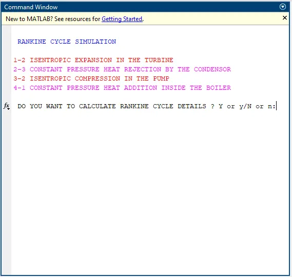
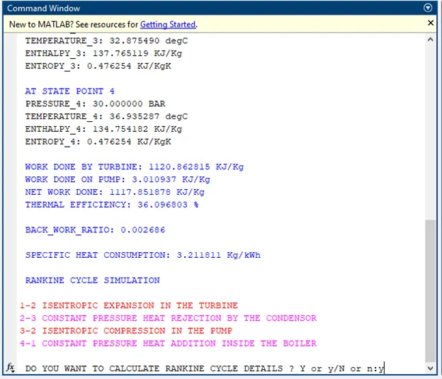
When user provides ‘y’ or Y, then the following screenshot is observed and user inputs the parameters for calculations.

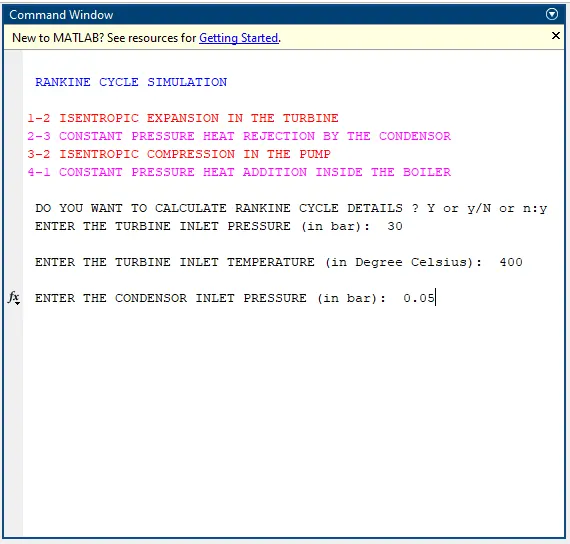
When enter is pressed on the computer keyboard, automatically, the output is generated . the below are the screen shots. All the state variables are determined are displayed in the command window for output.

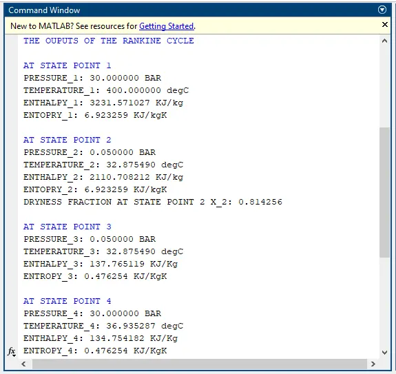
The below window has work done by turbine, work done on pump, net work done, thermal efficiency, back work ratio and specific heat consumption.

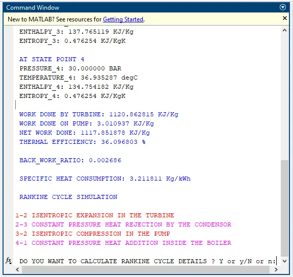
The above screenshot also asks user to are you interested to calculate Rankine cycle details. Before that I would be showing the Temperature Vs Entropy and Enthalpy Vs Entropy.

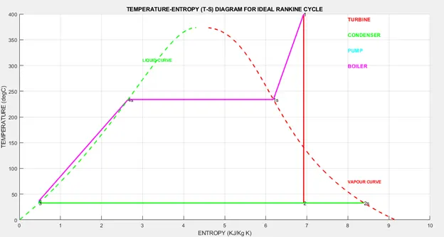
The above, plot describes, 1-2: isentropic expansion, and it is represented with red line where turbine works produce mechanical output to produce electricity. There is point 2s, which is generated due to saturation temperature and saturation vapor entropy. The dry saturated vapor expands through a turbine generating power. This decreases the temperature and pressure of the vapor, and some condensation may occur.

Rankine cycle is never been ideal cycle. As a result of irreversibilities in various components such as fluid friction and heat loss to the surroundings, the actual cycle deviates from the ideal Rankine cycle. The deviations of actual pumps and turbines from the isentropic ones. That’s reason the point 2s comes and the line joining from point 1 to point 2s won’t be vertical line and not isentropic.

The process covering state point form 2s, 2 to 3 is constant pressure heat rejection, this happens in condenser. Here, the vapor is condensed to liquid phase. This is represented by green color line. The wet vapor then enters a condenser, where it is condensed at a constant pressure to become a saturated liquid

The process between state points 3 to 4 is called isentropic compression where the entropy is constant, and the liquid phase is compressed to increase the pressure. As the fluid is a liquid at this stage, the working fluid is pumped from low to high pressure, so, it is done by pump or compressor, so some amount of energy is consumed by pump and it is loss in the process of work output produced at the end of turbine.

Once , the condensed fluid is pressurized is sent in to boiler, from state 4 to 4s and 1s, this process is called constant pressure heat addition, during which the heat addition takes places in steps to increase heat of the steam and it reached super-heated to produce good amount work and this is given input to the turbine. The high-pressure liquid enters a boiler, where it is heated at constant pressure by an external heat source to become a dry saturated vapor. The input energy required can be easily calculated graphically, using an entahlpy and entropy chart, or numerically, using steam table. This is represented by Magenta color. For this, I used ‘XSteam.m’ function.

The above picture has green dash ‘—’ line as liquid curve and red dash ‘—’ represents vapor curve. It is same in the enthalpy and entropy plot.

Correspondingly, enthalpy vs entropy plots are displayed. H-S diagram. The below is the screenshot of the plot.

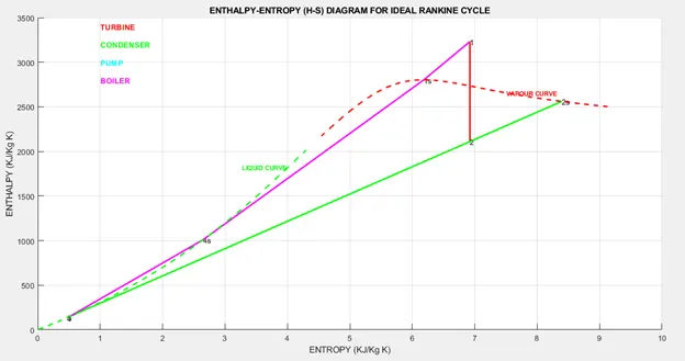
An enthalpy–entropy chart, also known as the H–S chart or Mollier diagram, plots the total heat against entropy, describing the enthalpy of a thermodynamic system. A typical chart covers a pressure range of 0.01–1000 bar, and temperatures up to 800 degreesCelsius. It shows enthalpy H in terms of internal energy U and pressure p and Volume V.

The work done in the Rankine cycle is represented by line from state point 1 to state point 2 of H-S diagram. So, work done represented by length of ‘H’, so, the difference between enthalpies at state 1 to state 2.

In an Isobaric process, the pressure remains constant, so the heat interaction is the change in enthalpy. In an isenthalpic process, the enthalpy is constant. A horizontal line in the diagram represents an isenthalpic process. Similar to the T-S diagram, red lines for turbine, green line for condenser, cyan for pump work, which is isenthalpic process and magenta is for fluid heat work in the boiler.

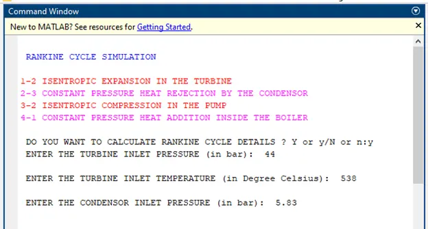
Now, again I pressed ‘y’ or ‘Y’ for the input in the command window, the following is the screenshot

As soon as , I entered after pressing ‘y’ or ‘Y’, all the previous plots are closed. Then I provide new parameters for calculations

The following are the output screenshots. When enter is pressed on the computer keyboard, automatically, the output is generated . the below are the screen shots. All the state variables are determined are displayed in the command window for output.

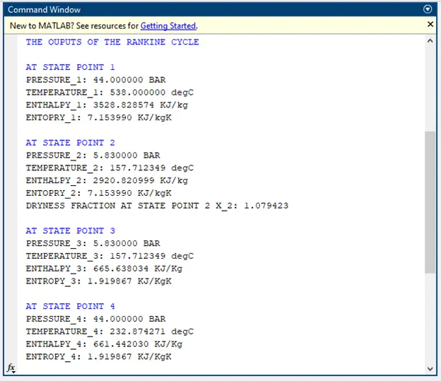
The below window has work done by turbine, work done on pump, net work done, thermal efficiency, back work ratio and specific heat consumption.

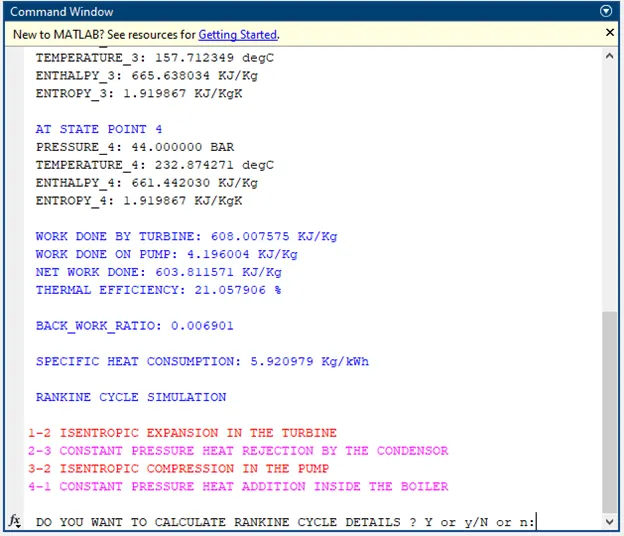
The following is T-S and H-S Diagram:

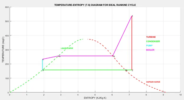
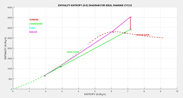
Now I press ‘n’ or ‘N’ as I don’t wish to calculate further so I get the below screenshot.

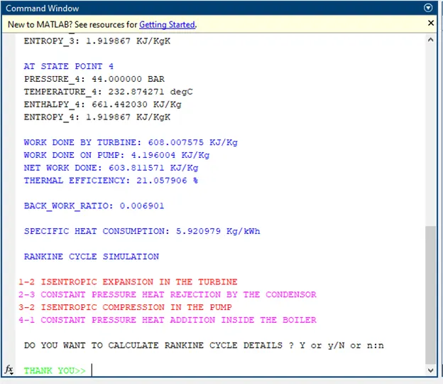
Finally , all the All the state variables are calculated are displayed in the command window for output and Plots of T-S and H-S diagram generated, simultaneously work done by turbine, work done on pump, net work done, thermal efficiency, back work ratio and specific heat consumption are displayed in command window.