Project 2 - Rankine cycle Simulator
A Rankine cycle simulator in MATLAB would simulate the thermodynamic Rankine cycle, which is a model of a steam-powered heat engine. The simulator would likely take input parameters such as the working fluid, the temperature and pressure at various points in the cycle, and the efficiency of the system. It would then use these inputs to calculate thermodynamic properties of the fluid and the performance of the cycle. The output of the simulator would likely include information such as the thermal efficiency, net power output, and heat input/output. It could also include plots of the thermodynamic states of the fluid during the cycle, such as temperature-entropy or pressure-volume diagrams.
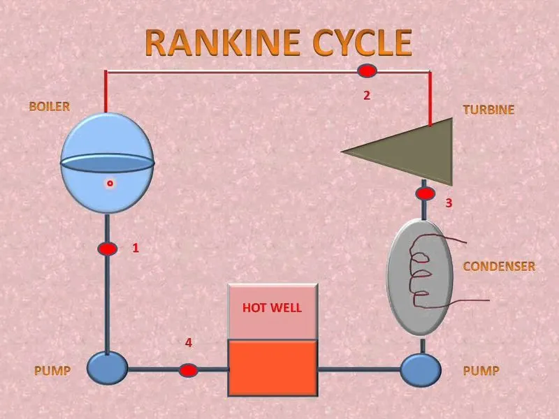
Code:
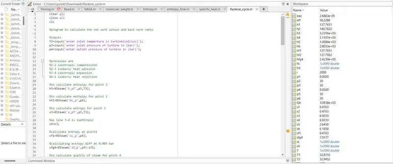
clear all
close all
clc
%program to calculate the net work outout and back work ratio
%inputs
T3=input('enter inlet temperture in turbine(celcius)');
p3=input('enter inlet pressure of turbine in (bar)');
p4=input('enter outlet pressure of turbine in (bar)');
%processes are
%1-2 isentropic comperession
%2-3 isobaric heat adission
%3-4 isentropic expansion
%4-1 isobsric heat rejection
%to calculate enthalpy for point 3
h3=XSteam('h_pT',p3,T3);
%to calculate enthalpy for point 1
hf1=XSteam('hL_p',p4);
%to calculate entropy for point 3
s3=XSteam('s_pT',p3,T3);
%as line 3-4 is isentropic
s4=s3;
%calculate entropy at point1
sf1=XSteam('sL_p',p4);
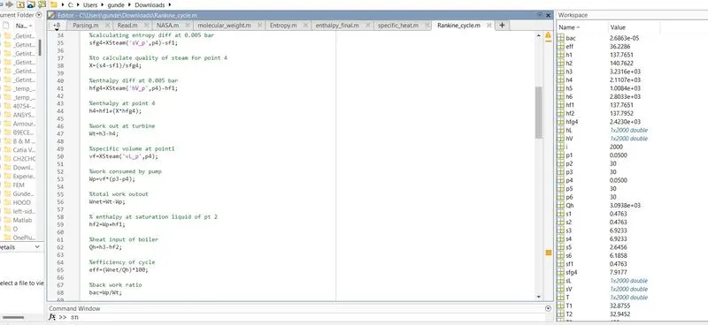
%calculating entropy diff at 0.005 bar
sfg4=XSteam('sV_p',p4)-sf1;
%to calculate quality of steam for point 4
X=(s4-sf1)/sfg4;
%enthalpy diff at 0.005 bar
hfg4=XSteam('hV_p',p4)-hf1;
%enthalpy at point 4
h4=hf1+(X*hfg4);
%work out at turbine
Wt=h3-h4;
%specific volume at point1
vf=XSteam('vL_p',p4);
%work consumed by pump
Wp=vf*(p3-p4);
%total work outout
Wnet=Wt-Wp;
% enthalpy at saturation liquid of pt 2
hf2=Wp+hf1;
%heat input of boiler
Qh=h3-hf2;
%efficiency of cycle
eff=(Wnet/Qh)*100;
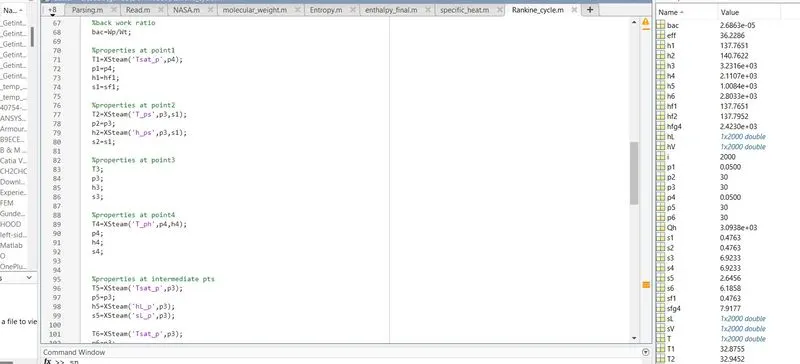
%back work ratio
bac=Wp/Wt;
%properties at point1
T1=XSteam('Tsat_p',p4);
p1=p4;
h1=hf1;
s1=sf1;
%properties at point2
T2=XSteam('T_ps',p3,s1);
p2=p3;
h2=XSteam('h_ps',p3,s1);
s2=s1;
%properties at point3
T3;
p3;
h3;
s3;
%properties at point4
T4=XSteam('T_ph',p4,h4);
p4;
h4;
s4;
%properties at intermediate pts
T5=XSteam('Tsat_p',p3);
p5=p3;
h5=XSteam('hL_p',p3);
s5=XSteam('sL_p',p3);
T6=XSteam('Tsat_p',p3);
p6=p3;
h6=XSteam('hV_p',p3);
s6=XSteam('sV_p',p3);
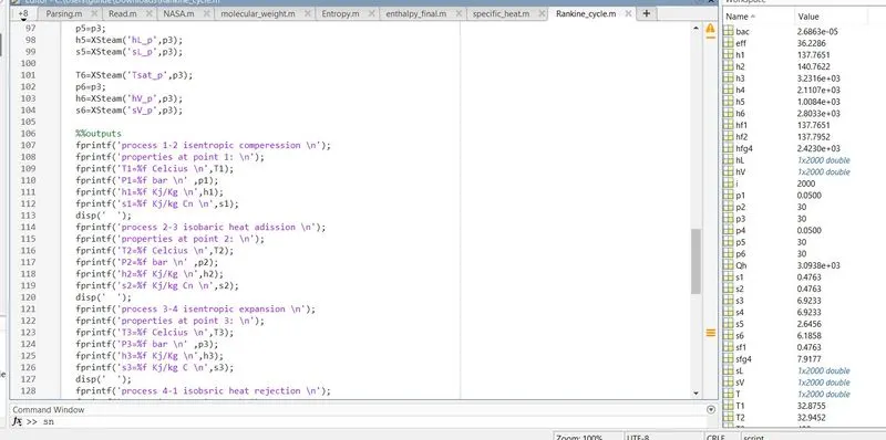
%%outputs
fprintf('process 1-2 isentropic comperession \n');
fprintf('properties at point 1: \n');
fprintf('T1=%f Celcius \n',T1);
fprintf('P1=%f bar \n' ,p1);
fprintf('h1=%f Kj/Kg \n',h1);
fprintf('s1=%f Kj/kg Cn \n',s1);
disp(' ');
fprintf('process 2-3 isobaric heat adission \n');
fprintf('properties at point 2: \n');
fprintf('T2=%f Celcius \n',T2);
fprintf('P2=%f bar \n' ,p2);
fprintf('h2=%f Kj/Kg \n',h2);
fprintf('s2=%f Kj/kg Cn \n',s2);
disp(' ');
fprintf('process 3-4 isentropic expansion \n');
fprintf('properties at point 3: \n');
fprintf('T3=%f Celcius \n',T3);
fprintf('P3=%f bar \n' ,p3);
fprintf('h3=%f Kj/Kg \n',h3);
fprintf('s3=%f Kj/kg C \n',s3);
disp(' ');
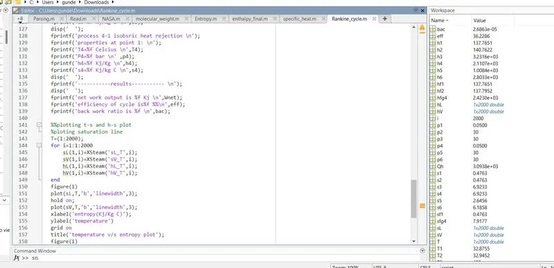
fprintf('process 4-1 isobsric heat rejection \n');
fprintf('properties at point 1: \n');
fprintf('T4=%f Celcius \n',T4);
fprintf('P4=%f bar \n' ,p4);
fprintf('h4=%f Kj/Kg \n',h4);
fprintf('s4=%f Kj/kg C \n',s4);
disp(' ');
fprintf('-----------results----------- \n');
disp(' ');
fprintf('net work output is %f Kj \n',Wnet);
fprintf('efficiency of cycle is%f %%\n',eff);
fprintf('back work ratio is %f \n',bac);
%%plotting t-s and h-s plot
%ploting saturation line
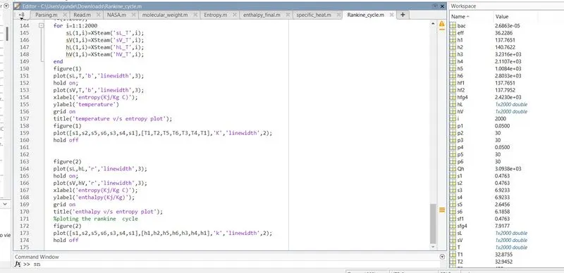
T=(1:2000);
for i=1:1:2000
sL(1,i)=XSteam('sL_T',i);
sV(1,i)=XSteam('sV_T',i);
hL(1,i)=XSteam('hL_T',i);
hV(1,i)=XSteam('hV_T',i);
end
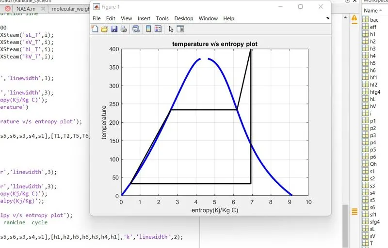
figure(1)
plot(sL,T,'b','linewidth',3);
hold on;
plot(sV,T,'b','linewidth',3);
xlabel('entropy(Kj/Kg C)');
ylabel('temperature')
grid on
title('temperature v/s entropy plot');
figure(1)
plot([s1,s2,s5,s6,s3,s4,s1],[T1,T2,T5,T6,T3,T4,T1],'K','linewidth',2);
hold off
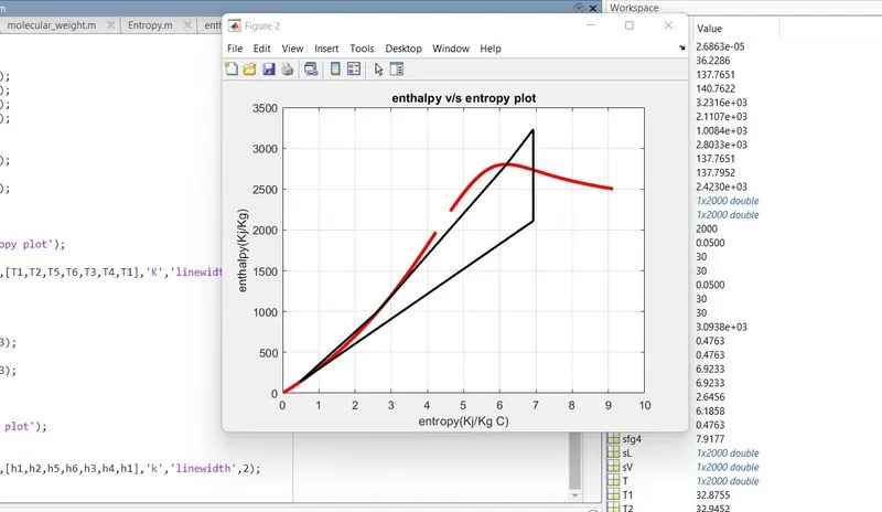
figure(2)
plot(sL,hL,'r','linewidth',3);
hold on;
plot(sV,hV,'r','linewidth',3);
xlabel('entropy(Kj/Kg C)');
ylabel('enthalpy(Kj/Kg)');
grid on
title('enthalpy v/s entropy plot');
%ploting the rankine cycle
figure(2)
plot([s1,s2,s5,s6,s3,s4,s1],[h1,h2,h5,h6,h3,h4,h1],'k','linewidth',2);
hold off
Result:
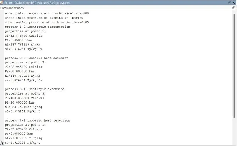
enter inlet temperture in turbine(celcius)400
enter inlet pressure of turbine in (bar)30
enter outlet pressure of turbine in (bar)0.05
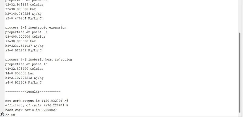
process 1-2 isentropic comperession
properties at point 1:
T1=32.875490 Celcius
P1=0.050000 bar
h1=137.765119 Kj/Kg
s1=0.476254 Kj/kg Cn
process 2-3 isobaric heat adission
properties at point 2:
T2=32.945189 Celcius
P2=30.000000 bar
h2=140.762226 Kj/Kg
s2=0.476254 Kj/kg Cn
process 3-4 isentropic expansion
properties at point 3:
T3=400.000000 Celcius
P3=30.000000 bar
h3=3231.571027 Kj/Kg
s3=6.923259 Kj/kg C
process 4-1 isobsric heat rejection
properties at point 1:
T4=32.875490 Celcius
P4=0.050000 bar
h4=2110.708212 Kj/Kg
s4=6.923259 Kj/kg C
-----------results-----------
net work output is 1120.832706 Kj
efficiency of cycle is36.228634 %
back work ratio is 0.000027
>>
enter inlet pressure of turbine in (bar)30
enter outlet pressure of turbine in (bar)0.05
process 1-2 isentropic comperession
properties at point 1:
T1=32.875490 Celcius
P1=0.050000 bar
h1=137.765119 Kj/Kg
s1=0.476254 Kj/kg Cn
process 2-3 isobaric heat adission
properties at point 2:
T2=32.945189 Celcius
P2=30.000000 bar
h2=140.762226 Kj/Kg
s2=0.476254 Kj/kg Cn
process 3-4 isentropic expansion
properties at point 3:
T3=400.000000 Celcius
P3=30.000000 bar
h3=3231.571027 Kj/Kg
s3=6.923259 Kj/kg C
process 4-1 isobsric heat rejection
properties at point 1:
T4=32.875490 Celcius
P4=0.050000 bar
h4=2110.708212 Kj/Kg
s4=6.923259 Kj/kg C
-----------results-----------
net work output is 1120.832706 Kj
efficiency of cycle is36.228634 %
back work ratio is 0.000027
>>
 clear all close all clc %program to calculate the net work outout and back work ratio %inputs T3=input('enter inlet temperture in turbine(celcius)'); p3=input('enter inlet pressure of turbine in (bar)'); p4=input('enter outlet pressure of turbine in (bar)'); %processes are %1-2 isentropic comperession %2-3 isobaric heat adissions %3-4 isentropic expansion %4-1 isobsric heat rejection %to calculate enthalpy for point 3 h3=XSteam('h_pT',p3,T3); %to calculate enthalpy for point 1 hf1=XSteam('hL_p',p4); %to calculate entropy for point 3 s3=XSteam('s_pT',p3,T3); %as line 3-4 is isentropic s4=s3; %calculate entropy at point1 sf1=XSteam('sL_p',p4); %calculating entropy diff at 0.005 bar sfg4=XSteam('sV_p',p4)-sf1; %to calculate quality of steam for point 4 X=(s4-sf1)/sfg4; %enthalpy diff at 0.005 bar hfg4=XSteam('hV_p',p4)-hf1; %enthalpy at point 4 h4=hf1+(X*hfg4); %work out at turbine Wt=h3-h4; %specific volume at point1 vf=XSteam('vL_p',p4); %work consumed by pump Wp=vf*(p3-p4); %total work outout Wnet=Wt-Wp; % enthalpy at saturation liquid of pt 2 hf2=Wp+hf1; %heat input of boiler Qh=h3-hf2; %efficiency of cycle eff=(Wnet/Qh)*100; %back work ratio bac=Wp/Wt; %properties at point1 T1=XSteam('Tsat_p',p4); p1=p4; h1=hf1; s1=sf1; %properties at point2 T2=XSteam('T_ps',p3,s1); p2=p3; h2=XSteam('h_ps',p3,s1); s2=s1; %properties at point3 T3; p3; h3; s3; %properties at point4 T4=XSteam('T_ph',p4,h4); p4; h4; s4; %properties at intermediate pts T5=XSteam('Tsat_p',p3); p5=p3; h5=XSteam('hL_p',p3); s5=XSteam('sL_p',p3); T6=XSteam('Tsat_p',p3); p6=p3; h6=XSteam('hV_p',p3); s6=XSteam('sV_p',p3); %%outputs fprintf('process 1-2 isentropic comperession \n'); fprintf('properties at point 1: \n'); fprintf('T1=%f Celcius \n',T1); fprintf('P1=%f bar \n' ,p1); fprintf('h1=%f Kj/Kg \n',h1); fprintf('s1=%f Kj/kg Cn \n',s1); disp(' '); fprintf('process 2-3 isobaric heat adission \n'); fprintf('properties at point 2: \n'); fprintf('T2=%f Celcius \n',T2); fprintf('P2=%f bar \n' ,p2); fprintf('h2=%f Kj/Kg \n',h2); fprintf('s2=%f Kj/kg Cn \n',s2); disp(' '); fprintf('process 3-4 isentropic expansion \n'); fprintf('properties at point 3: \n'); fprintf('T3=%f Celcius \n',T3); fprintf('P3=%f bar \n' ,p3); fprintf('h3=%f Kj/Kg \n',h3); fprintf('s3=%f Kj/kg C \n',s3); disp(' '); fprintf('process 4-1 isobsric heat rejection \n'); fprintf('properties at point 1: \n'); fprintf('T4=%f Celcius \n',T4); fprintf('P4=%f bar \n' ,p4); fprintf('h4=%f Kj/Kg \n',h4); fprintf('s4=%f Kj/kg C \n',s4); disp(' '); fprintf('-----------results----------- \n'); disp(' '); fprintf('net work output is %f Kj \n',Wnet); fprintf('efficiency of cycle is%f %%\n',eff); fprintf('back work ratio is %f \n',bac); %%plotting t-s and h-s plot %ploting saturation line T=(1:2000); for i=1:1:2000 sL(1,i)=XSteam('sL_T',i); sV(1,i)=XSteam('sV_T',i); hL(1,i)=XSteam('hL_T',i); hV(1,i)=XSteam('hV_T',i); end figure(1) plot(sL,T,'b','linewidth',3); hold on; plot(sV,T,'b','linewidth',3); xlabel('entropy(Kj/Kg C)'); ylabel('temperature') grid on title('temperature v/s entropy plot'); figure(1) plot([s1,s2,s5,s6,s3,s4,s1],[T1,T2,T5,T6,T3,T4,T1],'K','linewidth',2); hold off figure(2) plot(sL,hL,'r','linewidth',3); hold on; plot(sV,hV,'r','linewidth',3); xlabel('entropy(Kj/Kg C)'); ylabel('enthalpy(Kj/Kg)'); grid on title('enthalpy v/s entropy plot'); %ploting the rankine cycle figure(2) plot([s1,s2,s5,s6,s3,s4,s1],[h1,h2,h5,h6,h3,h4,h1],'k','linewidth',2); hold off