Project 2 - Rankine cycle Simulator
clear all
close all
clc

%information
fprintf('\n        RANKINE CYCLE SIMULATOR             ');
fprintf('\n\n1-2 Isentropic Expansion in Turbine');
fprintf('\n2-3 Constant Pressure Heat Rejection in the Condenser');
fprintf('\n3-4 Isentropic Compression in the Pump');
fprintf('\n4-1 Constant Pressure Heat Addition by the Boiler\n');

%inputs
p1=input(' Pressure at the Turbine inlet (bar) : ');
t1=input(' Temperature at the Turbine inlet (celsius) : ');
p2=input(' Pressure at the Condenser : ');


% @ stage 1 Turbine Inlet
% p1 & t1 are given
h1=XSteam('h_pT',p1,t1);
s1=XSteam('s_pT',p1,t1);

% @ stage 2 Condenser Inlet
%p2 is given
s2=s1;
sf2=XSteam('sL_p',p2);
sg2=XSteam('sV_p',p2);
hf2=XSteam('hL_p',p2);
hg2=XSteam('hV_p',p2);
x2=(s2-sf2)/(sg2-sf2);
h2=hf2+(x2*(hg2-hf2));

% @ stage 3 Pump Inlet
p3=p2;
h3=XSteam('hL_p',p3);
s3=XSteam('sL_p',p3);
t3=XSteam('Tsat_p',p3);
t2=t3;

% @ stage 4 Boiler Inlet
p4=p1;
s4=s3;
h4=XSteam('h_ps',p4,s4);

cp4=XSteam('Cp_ps',p4,s4);
cv4=XSteam('Cv_ps',p4,s4);
lambda=cp4/cv4;
t4=t3/((p3/p4)^((lambda-1)/lambda));

t5=XSteam('Tsat_p',p1);
t6=t5;
s5=XSteam('sL_p',p1);
s6=XSteam('sV_p',p1);
h5=XSteam('hL_p',p1);
h6=XSteam('hV_p',p1);


% Turbine Work
Wt=h1-h2;

% Pump Work
Wp=h4-h3;

% Net Work (kJ/Kg)
W=Wt-Wp;

% Heat in & out of the System
Q_in=h1-h4;
Q_out=h2-h3;

% Thermal Efficiency
ntherm=(W/Q_in)*100;

% Steam rate (kg/kWh)
SSC=3600/W;

% Back Work Ratio
BWR=(h1-h4)/(h2-h3);

% to plot Saturation Curve
T=linspace(1,400,500);
for i=1:length(T)
  h_l(i)=XSteam('hL_T',T(i));
  h_v(i)=XSteam('hV_T',T(i));
  s_l(i)=XSteam('sL_T',T(i));
  s_v(i)=XSteam('sV_T',T(i));
end

% plotting TS diagram
figure(1)
hold on
title('T-S Diagram')
plot([s1 s2],[t1 t2],'linewidth',3,'color','b')
plot([s2 s3],[t2 t3],'linewidth',3,'color','b')
plot([s3 s4],[t3 t4],'linewidth',3,'color','b')
plot([s4 s5],[t4 t5],'linewidth',3,'color','b')
plot([s5 s6],[t5 t6],'linewidth',3,'color','b')
xlabel('Entropy (kJ/KgK');
ylabel('Temperature (deg C)');
s_1=linspace(s6,s1,500);
for j=1:length(s_1)
  t_1(j)=XSteam('T_ps',p1,s_1(j));
end
plot(s_1,t_1,'linewidth',3,'color','b')
plot(s_l,T,'linewidth',1.5,'color','r')
plot(s_v,T,'linewidth',1.5,'color','r')
% Annotations
text(s1,t1,'1','fontsize',15);
text(s2,t2,'2','fontsize',15);
text(s3,t3,'3','fontsize',15,'verticalalignment','top');
text(s4,t4,'4','fontsize',15,'verticalalignment','bottom');
text(s5,t5,'5','fontsize',15,'verticalalignment','bottom');
text(s6,t6,'6','fontsize',15,'verticalalignment','bottom');

figure(2)
hold on
title('H-S Diagram');
plot([s1 s2],[h1 h2],'linewidth',2,'color','b')
plot([s2 s3],[h2 h3],'linewidth',2,'color','b')
plot([s3 s4],[h3 h4],'linewidth',2,'color','b')

h_4=linspace(h4,h5,500);
for k=1:length(h_4);
  s_4(k)=XSteam('s_ph',p1,h_4(k));
end

h_6=linspace(h6,h1,500);
for m=1:length(h_6);
  s_6(m)=XSteam('s_ph',p1,h_6(m));
end

plot(s_4,h_4,'linewidth',2,'color','b')
plot([s5 s6],[h5 h6],'linewidth',2,'color','b')
plot(s_6,h_6,'linewidth',2,'color','b')
xlabel('Specific Entropy (kJ/KgK)');
ylabel('Specific Enthalpy (kJ/Kg)');
plot(s_l,h_l,'linewidth',1.5,'color','r')
plot(s_v,h_v,'linewidth',1.5,'color','r')

% Annotations
text(s1,h1,'1','fontsize',15);
text(s2,h2,'2','fontsize',15);
text(s3,h3,'3','fontsize',15,'verticalalignment','top');
text(s4,h4,'4','fontsize',15,'verticalalignment','bottom');
text(s5,h5,'5','fontsize',15,'verticalalignment','bottom');
text(s6,h6,'6','fontsize',15,'verticalalignment','bottom');

% Results Window
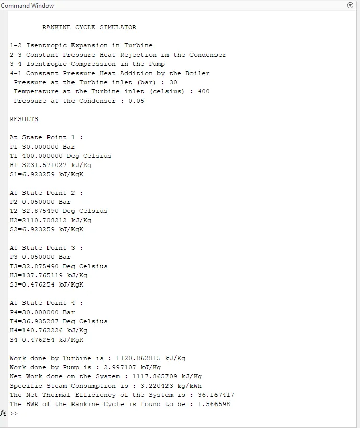
fprintf('\nRESULTS\n\n');
fprintf('At State Point 1 :\n');
fprintf('P1=%f Bar\n',p1);
fprintf('T1=%f Deg Celsius\n',t1);
fprintf('H1=%f kJ/Kg\n',h1);
fprintf('S1=%f kJ/KgK\n\n',s1);

fprintf('At State Point 2 :\n');
fprintf('P2=%f Bar\n',p2);
fprintf('T2=%f Deg Celsius\n',t2);
fprintf('H2=%f kJ/Kg\n',h2);
fprintf('S2=%f kJ/KgK\n\n',s2);

fprintf('At State Point 3 :\n');
fprintf('P3=%f Bar\n',p3);
fprintf('T3=%f Deg Celsius\n',t3);
fprintf('H3=%f kJ/Kg\n',h3);
fprintf('S3=%f kJ/KgK\n\n',s3);

fprintf('At State Point 4 :\n');
fprintf('P4=%f Bar\n',p4);
fprintf('T4=%f Deg Celsius\n',t4);
fprintf('H4=%f kJ/Kg\n',h4);
fprintf('S4=%f kJ/KgK\n\n',s4);

fprintf('Work done by Turbine is : %f kJ/Kg\n',Wt);
fprintf('Work done by Pump is : %f kJ/Kg\n',Wp);
fprintf('Net Work done on the System : %f kJ/Kg\n',W);
fprintf('Specific Steam Consumption is : %f kg/kWh\n',SSC);
fprintf('The Net Thermal Efficiency of the System is : %f\n',ntherm);
fprintf('The BWR of the Rankine Cycle is found to be : %f\n',BWR);
RESULTS---
PLOTS are attched.
CODE EXPLANATION----The Program begins with clear all, close all, clc to erase the workspace and plots.
A series of information on Rankine Cycle is processed to Comand window using fprintf comand.
Input variables P1,T1,P2 are given by input comand whose values are entered in comand window while executing the Program.
The data for the Rankine Cycle is extracted by the XSteam.m file which contains Water & Steam properties.
@State-1, Values for Enthalpy & Entropy are extracted as a function of Pressure & Temperature.
h_pT, s_pT, hL_p, sV_p etc.... are the default variables whose value is stored in XSteam file.
Similarly all the variables for all states are extracted using suitable format.
**The Formulae for the State Variables and other depending factors are referred from Power Plant Reference Books.
Pressure, Temperature, Enthalpy, Entropy forall the State Variables are Extracted as a function of dependent variable from the XSteam File.
@State 2 is an Condenser inlet where the High Pressure Steam is coverted into Low Pressure Water and hence Dryness Fraction, Enthalpy & Entropy for Saturated Vapour & Saturated Water are considered to Calculate the Specific Enthalpy.
@State-3 The water is condensed back to its Saturation Temperature and fed to the Pump, This temperature of water at the exit of the Condenser and entry of Pump is same.
@State-4 This is Constant Pressure Heat addition, hence pressure is equal to p1, but the temperature increases on heating at Constant Pressure & Constant Volume as our Entropy remains same and hence Cp/Cv=lambda is considered to find temperature T4.
Finally Work done and Heat Evolved & SSC are calculated by basic formulae.
To plot the Saturation Curve, a Temerature range is defined using linspace comand and for the overall length of this Temperature values of Enthalpy and Entropy are calculated at every temperature point. The Break in the Saturation Curve seperates the Liquid Phase & Vapour Phase.
Now all the necessary data is find out, Plotting is done for both T-S & H-S curves using the plot comands. Annotations are assigned using text comand.
Results of the Cycle Simulation is displayed over Comand window using fprintf comand.
Back Work Ratio (BWR) is defined as the fraction of the work produced by the turbine that is consumed by the pump. BWR should range from 1 to 2 for Vapour Power Cycle like Rankine.