Project 2 - Rankine cycle Simulator
AIM: Create a Rankine Cycle Simulator using MATLAB.
OBJECTIVE:
- Calculate each state points of the Rankine Cycle (any type of your choice) based on user inputs.
- Plot the corresponding T-s and h-s plots for the given set of inputs.
- Calculate Efficiency.
Theory:-
Rankine cycle is a model used to predict the performance of steam turbine systems.Rankine cycle consits of an operating fluid which continuously gets evaporated and condensed in a close loop.
Components used:-
Theory:-
The Rankine cycle is a model used to predict the performance of steam turbine systems.Rankine cycle consits of an operating fluid which continuously gets evaporated and condensed in a close loop.
Boiler
Turbine
Condenser
Pump
# Boiler for generating steam at constant pressure.
# turbine or engine in which steam will expand isentropically and work is done.
#condenser in which heat is removed from the exhaust steam and it is completely converted into water at constant pressure.
# pump which raises the pressure of liquid water to boiler pressure and pumps it in to the boiler for converting into steam.
Sample output of a Basic Rankine cycle simulator:
Process:
1-2: Isentropic compression in pump
2-3: Constant pressure heat addition in boiler
3-4: Isentropic expansion in turbine
4-1: Constant pressure heat rejection in condenser
code:
clear all
close all
clc

disp('RANKINE CYCLE SIMULATOR');
disp('1-2 = isentropic expansion in the turbine');
disp('2-3 = constant pressure heat rejection by the condensor');
disp('3-4 = isentropic compression in the pump');
disp('4-1 = constant pressure heat addition by the boiler');

%To type the inputs and getting the text as given in the problem

t1 = input('enter the temperature at the turbine inlet (in degree celsius):');

p1=input('enter the pressure at the turbine inlet (in bar):');
p2=input('enter the pressure at the condensor (in bar)');

fprintf('\rRESULTS\r\n')

%stage 1 (turbine inlet)
s1= XSteam('s_pT',p1,t1);
h1=XSteam('h_pT',p1,t1);

%stage 2 condenser inlet
sf2 = XSteam('sL_p',p2);
sg2 = XSteam('sV_p',p2);
hf2 = XSteam('hL_p',p2);
hg2 = XSteam('hV_p',p2);

s2 = s1;
t2 = XSteam('Tsat_p',p2);

%splitting the formulae

x2=((s2-sf2)/(sg2-sf2));
h2=hf2+(x2*(hg2-hf2));

%stage3 (pump inlet)
p3=p2;
t3=XSteam('Tsat_p',p2);
s3=XSteam('sL_p',p3);
h3=XSteam('hL_p',p3);

cp4 = XSteam('cpL_p',p3);
cv4 = XSteam('cvL_p',p3);
gamma = (cp4/cv4);
g = (gamma-1)/gamma;

%stage 4(boiler inlet)

p4=p1;
s4=s3;
h4 = XSteam('h_ps',p4,s4);
t4=t3*((p4/p3)^g);

%turbine work
wt=h1-h2;
%pump work
wp=h4-h3;
%network
w_net=wt-wp;

%Heat in and out of the system
q_in=h1-h4;
q_out=h2-h3;

q_in=h1-h4;
q_out=h2-h3;

n=w_net/q_in;
np=n*100;

SSC=3600/w_net;
tf_sat=XSteam('Tsat_p',p1);
sf_sat=XSteam('sL_p',p1);
hf_sat=XSteam('hL_p',p1);
sg_sat=XSteam('sV_p',p1);
hg_sat=XSteam('hV_p',p1);

%plot figure 1
figure(1)
hold on
temp=linspace(0,400,1000);
for i=1:length(temp)
    aa(i) =XSteam('sL_T',temp(i));

end

for j=1:length(temp)
    bb(j)=XSteam('sV_T',temp(j));
end

plot(aa,temp,'color','b')
plot(bb,temp,'color','b')

temp=(XSteam('Tsat_p',p1));
t0=linspace(temp,t1,300);
for i=1:length(t0)
    c11(i)=XSteam('s_pt',p1,t0(i));
end

t5=XSteam('Tsat_p',p4);
s5=XSteam('sL_T',t5);

plot([s1 s2],[t1 t2],'color','r')
plot([s2 s3],[t2 t3],'color','r')
plot([s3 s4],[t3 t4],'color','r')
plot([s4 s5],[t4 t5],'color','r')
plot([sf_sat sg_sat],[tf_sat tf_sat],'color','r')
plot(c11,t0,'color','r')

title('T-S diagram')
xlabel('entropy(KJ/kgK)')
ylabel('Temperature(K)')

text(s1,t1,'1');
text(s2,t2,'2');
text(s3,t3,'3');
text(s4,t4,'4');
text(s5,t5,'4s');
text(sg_sat,tf_sat,'1s');

%plotting figure 2
figure(2)
hold on

temp1=linspace(0,400,1000);
for i=1:length(temp1)
    cc(i)=XSteam('hL_T',temp1(i));
end

for j=1:length(temp1)
    dd(j)=XSteam('hV_T',temp1(j));

end

plot(aa,cc,'color','b')
plot(bb,dd,'color','b')

plot([s1 s2],[h1 h2],'color','r')
plot([s2 s3],[h2 h3],'color','r')
plot([s3 s4],[h3 h4],'color','r')
plot([s4 s1],[h4 h1],'color','r')


title('H-S diagram')
xlabel('entropy(KJ/KgK)')
ylabel('enthalpy(KJ/Kg)')

text(s1,h1,'1');
text(s2,h2,'2');
text(s3,h3,'3');
text(s4,h4,'4');

%printing the output

fprintf('at stage point 1:\n')
fprintf('P1 is : %f bar\n',p1)
fprintf('T1 is : %f deg celsius\n',p1)
fprintf('T1 is :%f KJ/kg\n',h1)
fprintf('S1 is: %f KJ/KgK\r\n',s1)

disp('at state point 2:')
fprintf('P2 is : %f Bar\n',p2)
fprintf('T2 is : %f deg celsius\n',t2)
fprintf('H2 is : %f KJ/Kg\n',h2)
fprintf('S2 is : %f KJ/KgK\n',s2)
fprintf('X is : %f \r\n',x2)


disp('at state point 3:')
fprintf('P3 is : %f Bar\n',p3)
fprintf('T3 is : %f deg celsius400\n',t3)
fprintf('H3 is : %f KJ/Kg\n',h3)
fprintf('S2 is : %f KJ/KgK\b\n',s3)


disp('at state point 4:')
fprintf('P4 is : %f Bar\n',p4)
fprintf('T4 is : %f deg celsius\n',t4)
fprintf('H4 is : %f KJ/Kg\n',h4)
fprintf('S4 is : %f KJ/KgK\b\n',s4)

fprintf('Wt : %f KJ/Kg\n',wt)
fprintf('Wp : %f KJ/Kg\n',wp)
fprintf('Wnet : %f KJ/Kg\n',w_net)
fprintf('Ntherm : %f %%\n',n*100)
fprintf('SSC : %f KJ/KWh\b\n',SSC)
Result:
T-S Diagram
H-S Diagram
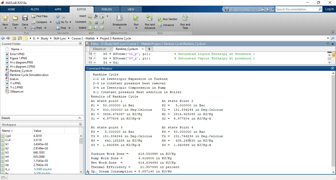
The values for the state point in command windows are given as:
For Inlet pressure in Turbine as = 50 bar
Inlet temperature in Turbine = 500 deg.cel
Pressure in condenser = 5 bar
For Input given in challeng:
For Inlet pressure in Turbine as = 30 bar
Inlet temperature in Turbine = 400 deg.cel
Pressure in condenser = 0.05 bar
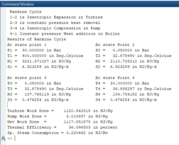
From the two different input value it is seen that increasing the pressure and temperature in turbine result in lowering the efficiency of Rankine cycle.
Conclusion:
I have created the Rankine cycle simulator for the given input, in which we have taken the data from XSteam function file.