Project 2 - Rankine cycle Simulator
% Rankine Cycle Simulator
close all
clc
% Printing Introduction
fprintf('RANKINE CYCLE SIMULATOR')
fprintf('1-2 is isentropic expansion in the Turbine')
fprintf('2-3 is Constant Pressure Heat Rejection by the Condenser')
fprintf('3-4 is isentropic Compression in pump')
fprintf('4-1 is Constant Pressure Heat Addition by the Boiler')
% User Inputs
P1 = input('Enter the Pressure at the Turbine Inlet (in bar):');
T1 = input('Enter the Temprature at the Turbine Inlet (in Degree Celcius):');
P2 = input('Enter the Pressure at the Turbine Outlet (in bar):');
% State point 1
H1 = XSteam('h_pt',P1,T1); %Enthalpy
S1 = XSteam('s_pt',P1,T1); %Entropy
Hf1 = XSteam('hL_p',P1); %Enthalpy of saturated liquid
Hg1 = XSteam('hV_p',P1); %Enthaply of saturated vapour
Ts1 = XSteam('Tsat_p',P1); %Saturation Temprature
Sf1 = XSteam('sL_p',P1); %Entropy of saturated liquid
Sg1 = XSteam('sV_p',P1); %Entropy of saturated vapour
% State point 2
S2 = S1;
Sf2 = XSteam('sL_p',P2);
Sg2 = XSteam('sV_p',P2);
x = (S2-Sf2)/(Sg2-Sf2); % Dryness fraction
Hf2 = XSteam('hL_p',P2);
Hg2 = XSteam('hV_p',P2);
H2 = Hf2 + x*(Hg2-Hf2);
T2 = XSteam('T_ph',P2,H2);
Ts2 = XSteam('Tsat_p',P2);
% State point 3
H3 = Hf2;
S3 = Sf2;
T3 = T2;
P3 = P2;
% State point 4
P4 = P1;
S4 = S3;
H4 = XSteam('h_ps',P4,S4);
T4 = XSteam('T_ps',P4,S4);
t = linspace(0,374,500); % temp space for plotting saturation cutves
%Plot T-S Diagram
figure(1)
hold on
% Plot Saturation Curve
for i = 1 : length(t)
plot(XSteam('sL_T',t(i)),t(i),'.','color','b')
plot(XSteam('sV_T',t(i)),t(i),'.','color','b')
end
% Plot Cycle
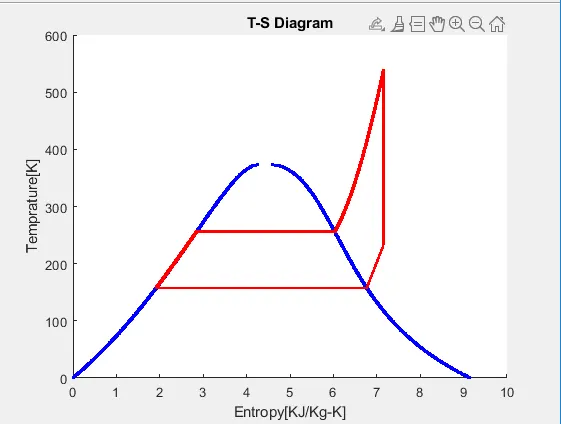
plot([S1 S2],[T1 T2],'linewidth',2,'color','r')
if x>1
T3 = Ts2;
plot([S2 Sg2 S3 S4],[T2 Ts2 T3 T4],'linewidth',2,'color','r')
T2 = Ts2;
else
plot([S2 S3 S4],[T2 T3 T4],'linewidth',2,'color','r')
end
l = linspace(T1,T2,1000);
for i = 1 : length(l)
plot(XSteam('s_pT',P1,l(i)),l(i),'.','color','r')
end
plot([Sf1 Sg1],[Ts1 Ts1],'linewidth',2,'color','r')
xlabel('Entropy[KJ/Kg-K]')
ylabel('Temprature[K]')
title('T-S Diagram')
% Plot H-S Diagram
figure(2)
hold on
% Plot Saturation Curve
for i = 1 : length(t)
plot(XSteam('sL_T',t(i)),XSteam('hL_T',t(i)),'.','color','b')
plot(XSteam('sV_T',t(i)),XSteam('hV_T',t(i)),'.','color','b')
end
% Plot Cycle
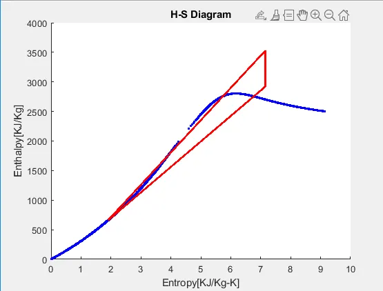
plot([S1 S2 S3 S4 S1],[H1 H2 H3 H4 H1],'linewidth',2,'color','r')
xlabel('Entropy[KJ/Kg-K]')
ylabel('Enthalpy[KJ/Kg]')
title('H-S Diagram')
% calculations
% Turbine Work
Wt = H1-H2;
% Pump Work
Wp = H4-H3;
% Heat Addition
Qin = H1-H4;
% Heat Rejection
Qout = H2-H3;
% Net Work
Wnet = Wt-Wp;
% Efficiency
Ntherm = (Wnet/Qin)*100;
% Specific steam consumption
SSC = 3600/Wnet;
% Back Work Ratio
BWR = Wp/Wt;
% Print Results
fprintf('Results')
fprintf('At State Point 1:')
fprintf('P1 is : %.2f bar',P1)
fprintf('T1 is : %.2f Deg Celcius',T1)
fprintf('H1 is : %.2f KJ/Kg',H1)
fprintf('S1 is : %.2f KJ/Kg-K',S1)
fprintf('\\nAt State Point 2:')
fprintf('P2 is : %.2f bar',P2)
fprintf('T2 is : %.2f Deg Celcius',T2)
fprintf('H2 is : %.2f KJ/Kg',H2)
fprintf('S2 is : %.2f KJ/Kg-K',S2)
fprintf('\\nAt State Point 3:')
fprintf('P3 is : %.2f bar',P3)
fprintf('T3 is : %.2f Deg Celcius',T3)
fprintf('H3 is : %.2f KJ/Kg',H3)
fprintf('S3 is : %.2f KJ/Kg-K',S3)
fprintf('\\nAt State Point 4:')
fprintf('P4 is : %.2f bar',P4)
fprintf('T4 is : %.2f Deg Celcius',T4)
fprintf('H4 is : %.2f KJ/Kg',H4)
fprintf('S4 is : %.2f KJ/Kg-K',S4)
fprintf('\\nWt is : %.2f KJ/Kg',Wt)
fprintf('Wp is : %.2f KJ/Kg',Wp)
fprintf('Wnet is : %.2f KJ/Kg',Wnet)
fprintf('Thermal Efficiency is : %.2f percent',Ntherm)
fprintf('S.S.C. is : %.2f Kg/KWh',SSC)
fprintf('Back Work Ratio is : %.3f',BWR)
#COMMAND WINDOW
RANKINE CYCLE SIMULATOR1-2 is isentropic expansion in the Turbine2-3 is Constant Pressure Heat Rejection by the Condenser3-4 is isentropic Compression in pump4-1 is Constant Pressure Heat Addition by the BoilerEnter the Pressure at the Turbine Inlet (in bar):44
Enter the Temprature at the Turbine Inlet (in Degree Celcius):538
Enter the Pressure at the Turbine Outlet (in bar):5.83
ResultsAt State Point 1:P1 is : 44.00 barT1 is : 538.00 Deg CelciusH1 is : 3528.83 KJ/KgS1 is : 7.15 KJ/Kg-K\nAt State Point 2:P2 is : 5.83 barT2 is : 157.71 Deg CelciusH2 is : 2920.82 KJ/KgS2 is : 7.15 KJ/Kg-K\nAt State Point 3:P3 is : 5.83 barT3 is : 157.71 Deg CelciusH3 is : 665.64 KJ/KgS3 is : 1.92 KJ/Kg-K\nAt State Point 4:P4 is : 44.00 barT4 is : 158.16 Deg CelciusH4 is : 669.84 KJ/KgS4 is : 1.92 KJ/Kg-K\nWt is : 608.01 KJ/KgWp is : 4.20 KJ/KgWnet is : 603.81 KJ/KgThermal Efficiency is : 21.12 percentS.S.C. is : 5.96 Kg/KWhBack Work Ratio is : 0.007>>