To create a program that simulates the state points of a rankine cycle from the inputs by user ad calculates the peformance parameters such as thermal efficiency, Back work ratio, turbine and pump work.
The Rankine cycle or Rankine vapour cycle is the process widely used for coal fired power plants or neuclear powerplants.In this the fuel is used to produce heat in the boiler that converts water to steam at high temperature and pressure which inturn drives the steam turbine.
Since water is used as the working fluid the efficiency of rankine cycle is limited due to the high heat of vapourization of water. The working fluid is to be recycled and reused constantly.
clear all
close all
clc
disp('RANKINE CYCLE SIMULATOR');
disp('1-2 = isentropic expansion in the turbine');
disp('2-3 = constant pressure heat rejection by the condensor');
disp('3-4 = isentropic compression in the pump');
disp('4-1 = constant pressure heat addition by the boiler');
%To type the inputs and getting the text as given in the problem
t1 = input('enter the temperature at the turbine inlet (in degree celsius):');
p1=input('enter the pressure at the turbine inlet (in bar):');
p2=input('enter the pressure at the condensor (in bar)');
fprintf('\rRESULTS\r\n')
%stage 1 (turbine inlet)
s1=XSteam('s_pT',p1,t1);
h1=XSteam('h_pT',p1,t1);
%stage 2 condenser inlet
sf2 = XSteam('sL_p',p2);
sg2 = XSteam('sV_p',p2);
hf2 = XSteam('hL_p',p2);
hg2 = XSteam('hV_p',p2);
s2 = s1;
t2 = XSteam('Tsat_p',p2);
%splitting the formulae
x2=((s2-sf2)/(sg2-sf2));
h2=hf2+(x2*(hg2-hf2));
%stage3 (pump inlet)
p3=p2;
t3=XSteam('Tsat_p',p2);
s3=XSteam('sL_p',p3);
h3=XSteam('hL_p',p3);
cp4 = XSteam('cpL_p',p3);
cv4 = XSteam('cvL_p',p3);
gamma = (cp4/cv4);
g = (gamma-1)/gamma;
%stage 4(boiler inlet)
p4=p1;
s4=s3;
h4 = XSteam('h_ps',p4,s4);
t4=t3*((p4/p3)^g);
%turbine work
wt=h1-h2;
%pump work
wp=h4-h3;
%network
w_net=wt-wp;
%Heat in and out of the system
q_in=h1-h4;
q_out=h2-h3;
q_in=h1-h4;
q_out=h2-h3;
n=w_net/q_in;
np=n*100;
SSC=3600/w_net;
tf_sat=XSteam('Tsat_p',p1);
sf_sat=XSteam('sL_p',p1);
hf_sat=XSteam('hL_p',p1);
sg_sat=XSteam('sV_p',p1);
hg_sat=XSteam('hV_p',p1);
%plot figure 1
figure(1)
hold on
temp=linspace(0,400,1000);
for i=1:length(temp)
aa(i) =XSteam('sL_T',temp(i));
end
for j=1:length(temp)
bb(j)=XSteam('sV_T',temp(j));
end
plot(aa,temp,'color','b')
plot(bb,temp,'color','b')
temp=(XSteam('Tsat_p',p1));
t0=linspace(temp,t1,300);
for i=1:length(t0)
c11(i)=XSteam('s_pt',p1,t0(i));
end
t5=XSteam('Tsat_p',p4);
s5=XSteam('sL_T',t5);
plot([s1 s2],[t1 t2],'color','r')
plot([s2 s3],[t2 t3],'color','r')
plot([s3 s4],[t3 t4],'color','r')
plot([s4 s5],[t4 t5],'color','r')
plot([sf_sat sg_sat],[tf_sat tf_sat],'color','r')
plot(c11,t0,'color','r')
title('T-S diagram')
xlabel('entropy(KJ/kgK)')
ylabel('Temperature(K)')
text(s1,t1,'1');
text(s2,t2,'2');
text(s3,t3,'3');
text(s4,t4,'4');
text(s5,t5,'4s');
text(sg_sat,tf_sat,'1s');
%plotting figure 2
figure(2)
hold on
temp1=linspace(0,400,1000);
for i=1:length(temp1)
cc(i)=XSteam('hL_T',temp1(i));
end
for j=1:length(temp1)
dd(j)=XSteam('hV_T',temp1(j));
end
plot(aa,cc,'color','b')
plot(bb,dd,'color','b')
plot([s1 s2],[h1 h2],'color','r')
plot([s2 s3],[h2 h3],'color','r')
plot([s3 s4],[h3 h4],'color','r')
plot([s4 s1],[h4 h1],'color','r')
title('H-S diagram')
xlabel('entropy(KJ/KgK)')
ylabel('enthalpy(KJ/Kg)')
text(s1,h1,'1');
text(s2,h2,'2');
text(s3,h3,'3');
text(s4,h4,'4');
%printing the output
fprintf('at stage point 1:\n')
fprintf('P1 is : %f bar\n',p1)
fprintf('T1 is : %f deg celsius\n',p1)
fprintf('T1 is :%f KJ/kg\n',h1)
fprintf('S1 is: %f KJ/KgK\r\n',s1)
disp('at state point 2:')
fprintf('P2 is : %f Bar\n',p2)
fprintf('T2 is : %f deg celsius\n',t2)
fprintf('H2 is : %f KJ/Kg\n',h2)
fprintf('S2 is : %f KJ/KgK\n',s2)
fprintf('X is : %f \r\n',x2)
disp('at state point 3:')
fprintf('P3 is : %f Bar\n',p3)
fprintf('T3 is : %f deg celsius400\n',t3)
fprintf('H3 is : %f KJ/Kg\n',h3)
fprintf('S2 is : %f KJ/KgK\b\n',s3)
disp('at state point 4:')
fprintf('P4 is : %f Bar\n',p4)
fprintf('T4 is : %f deg celsius\n',t4)
fprintf('H4 is : %f KJ/Kg\n',h4)
fprintf('S4 is : %f KJ/KgK\b\n',s4)
fprintf('Wt : %f KJ/Kg\n',wt)
fprintf('Wp : %f KJ/Kg\n',wp)
fprintf('Wnet : %f KJ/Kg\n',w_net)
fprintf('Ntherm : %f %%\n',n*100)
fprintf('SSC : %f KJ/KWh\b\n',SSC)
The following code does the following:
- Initially, it takes in values for the inlet, outlet conditions of turbine and boiler temperature
- Then it calculates the entropy for second state point as expansion in turbine is isentropic. values for entropies and other data in the code is exported fromthe XSteam.m file given.
- using the obtained data entropy at third state point is known with which entropy at boiler inlet is also obtained as pump in an isentropic process
- Similarly values for enthalpy is also found out.
- using the appropriate formulas and the data generated the performance parameters of the rankine cycle is found out.
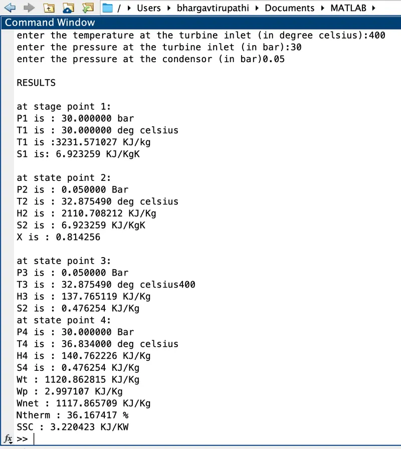
- The required data as asked is printed as output.
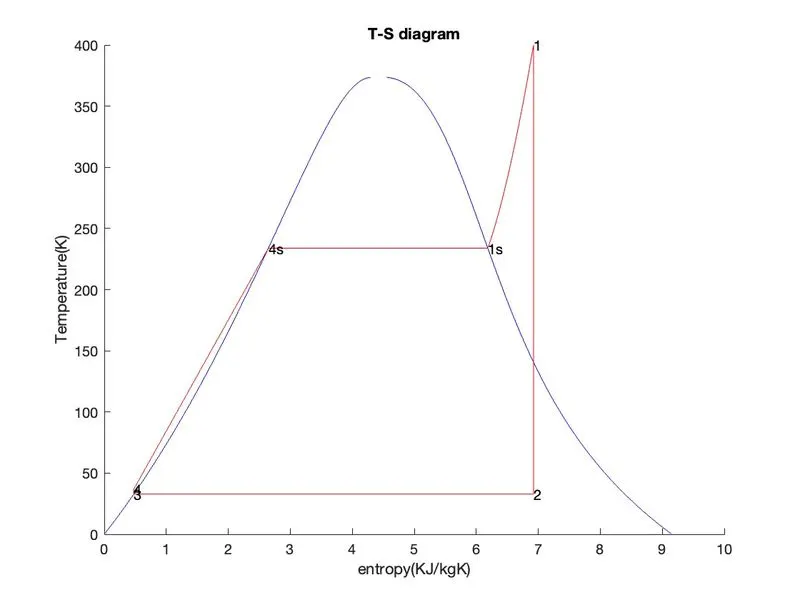
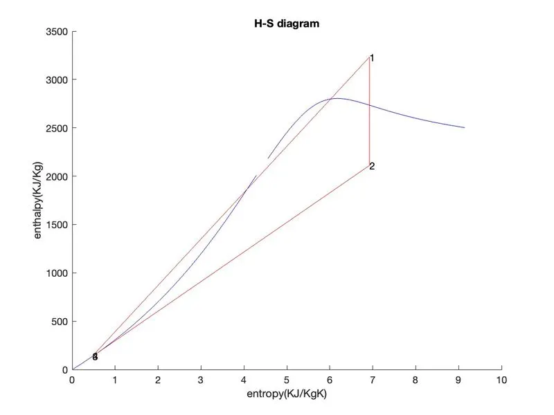
- For plotting of T-S diagram : isentropic process and constant pressure heat addition and rejection at latent heat temperature follow a straight line. So, can be plotted with two end points
- For constant pressure heat addition and rejection at sensible heat temperatures it follows the constant pressure line hence data is to be generated at each point. This is done by making use of a for loop
- Finally if the dryness fraction is grater than one at turbine outlet condition then heat rejection in condensor will initially follow the constant pressure curve until it reaches the saturation vapour temperature. if less than one the steam is wet in condition.
Results: