Project 2 - Rankine cycle Simulator
MAIN CODE


close all
clc

disp("      RANKIN CYCLE SUMILAROR    ")
disp("1-2 is iscentropic expantion in turbain")
disp("2-3 is constant pressure heat rejection by conduser")
disp("3-4 is icentropic compression is pump")
disp("4-1 is constant pressure heat addation at boiler")
p1=input("\nENTER THE PRESSURE AT TURBAIN INLET(in bar): ");
t1=input("ENTER THE TEMPRATURE AT TURBAIN INLET(in Dc): ");
p2=input("ENTER THE PRESSUERE AT CONDUNCER(in bar): ");

%CALCULATION
%state point 1
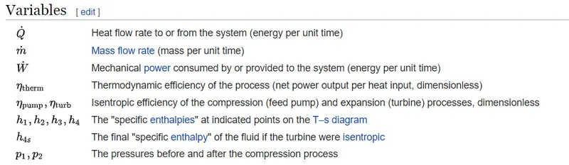
h1=XSteam('h_pT',p1,t1);
s1=XSteam('s_pT',p1,t1); %p1=high pressure

%state point 2
s2=s1;
sf2=XSteam('sL_p',p2); % L= liquid         sf=specific entropy of fluid
sg2=XSteam('sV_p',p2); % V= vapour         sg=specific entropy of liquide
hf2=XSteam('hL_p',p2);                    %hf=specific enthalpy of fluid
hg2=XSteam('hV_p',p2); %p2=low pressure    hg=specific enthalpy of liquid

%Dryness fraction
x2=((s2-sf2)/(sg2-sf2));

h2=hf2+(x2*(hg2-hf2));

%state point 3
p3=p2;
h3=XSteam('hL_p',p3);
s3=XSteam('sL_p',p3);
v3=XSteam('vL_p',p3);  % voloum
t3=XSteam('Tsat_p',p3);
t2=t3;

%state point 4
p4=p1;
s4=s3;
cp4=XSteam('cp_ps',p4,s4);
cv4=XSteam('cv_ps',p4,s4);
%gama
g=cp4/cv4;
o=(g-1)/g;
t4=t3*((p4/p3)^o);

%workdown by pump
wp=v3*(p4-p3)*100;

h4=h3+wp;

%Workdown by turbain
wt=h1-h2;

%net workdone
wnet=wt-wp;
%heat supplyed
q_in=h1-h4;
q_out=h2-h3;

%theromal efficiency
Nthermo=wnet/q_in;

% steam conducitivity
steam_rate=3600/(wt-wp);

%back work ratio
bwr=wp/wt;

%state point 5 & 6

t5=XSteam('Tsat_p',p1);
t6=t5;
if (t6==0)
    printf("the cycle connot have %f as inlet temprature !!!!")
end

s5=XSteam('sL_p',p1);
s6=XSteam('sL_p',p1);
h5=XSteam('hL_p',p1);
h6=XSteam('hL_p',p1);

sprintf('\n------------------RESULT------------------\n')
sprintf('At State point 1:\\np1 is : %4.2f Bar\\nt1 is : %4.2f Degree Celcius\\nh1 is : %4.2f kJ/kg\\ns1 is : %4.2f kJ/kgk\\n\\n\',p1,t1,h1,s1)
sprintf('At State point 2:\\np2 is : %4.2f Bar\\nt2 is : %4.2f Degree Celcius\\nh2 is : %4.2f kJ/kg\\ns2 is : %4.2f kJ/kgk\\n\\n\',p2,t2,h2,s2)
sprintf('At State point 3:\\np3 is : %4.2f Bar\\nt3 is : %4.2f Degree Celcius\\nh3 is : %4.2f kJ/kg\\ns3 is : %4.2f kJ/kgk\\n\\n\',p3,t3,h3,s3)
sprintf('At State point 4:\\np4 is : %4.2f Bar\\nt4 is : %4.2f Degree Celcius\\nh4 is : %4.2f kJ/kg\\ns4 is : %4.2f kJ/kgk\\n\\n\',p4,t4,h4,s4)
sprintf('wt is :%4.2f kJ/kg\\nwp is : %4.2f kJ/kg\\nwnet is : %4.2f kJ/kg\\nNthermo is : %4.2f percent\\nS.S.C is : %4.2f kg/kWh\',wt,wp,wnet,Nthermo,steam_rate)

warning off
t=linspace(1,500,1000);

%ploting T-S digram
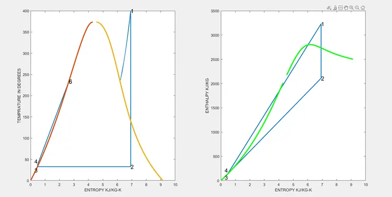
subplot(1,2,1)
t_rank=linspace(t5,t1,5000);
for i=1:length(t_rank)
    s_rank(i)=XSteam('s_pT',p1,t_rank(i));
end

plot([s1 s2 s3 s4 s5 s6 s_rank],[t1 t2 t3 t4 t5 t6 t_rank],'LineWidth',1.5);
hold on
t_curve=linspace(1,400,500);
for i=1:length(t_curve)
    s_l(i)=XSteam('sL_T',t_curve(i));
    s_v(i)=XSteam('sV_T',t_curve(i));
    h_l(i)=XSteam('hL_T',t_curve(i));
    h_v(i)=XSteam('hV_T',t_curve(i));
end

plot(s_l,t_curve,'LineWidth',3);
plot(s_v,t_curve,'LineWidth',3);
text(s1,t1,'1','FontSize',15)
text(s2,t2,'2','FontSize',15)
text(s3,t3,'3','FontSize',15,'HorizontalAlignment','right','VerticalAlignment','top')
text(s4,t4,'4','FontSize',15,'HorizontalAlignment','right','VerticalAlignment','bottom')
text(s5,t5,'5','FontSize',15)
text(s6,t6,'6','FontSize',15)
xlabel('ENTROPY KJ/KG-K')
ylabel('TEMPRATURE IN DEGREES')

%PLOT H-S DIGRAM
subplot(1,2,2);
plot([s1 s2 s3 s4 s1],[h1 h2 h3 h4 h1],'LineWidth',2);
hold on
plot(s_v,h_v,'linewidth',3,'Color','g');
plot(s_l,h_l,'linewidth',3,'color','g');
text(s1,h1,'1','FontSize',15)
text(s2,h2,'2','FontSize',15)
text(s3,h3,'3','FontSize',15,'HorizontalAlignment','right','VerticalAlignment','top')
text(s4,h4,'4','FontSize',15,'HorizontalAlignment','right','VerticalAlignment','bottom')
xlabel('ENTROPY KJ/KG-K')
ylabel('ENTHALPY KJ/KG')
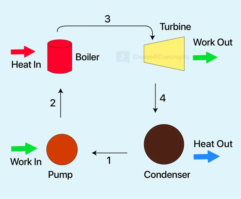
The Rankine cycle is an idealized thermodynamic cycle describing the process by which certain heat engines, such as steam turbines or reciprocating steam engines, allow mechanical work to be extracted from a fluid as it moves between a heat source and heat sink. The Rankine cycle is named after William John Macquorn Rankine, a Scottish polymath professor at Glasgow University.
Heat energy is supplied to the system via a boiler where the working fluid (typically water) is converted to a high pressure gaseous state (steam) in order to turn a turbine. After passing over the turbine the fluid is allowed to condense back into a liquid state as waste heat energy is rejected before being returned to boiler, completing the cycle. Friction losses throughout the system are often neglected for the purpose of simplifying calculations as such losses are usually much less significant than thermodynamic losses, especially in larger systems.
The Rankine cycle closely describes the process by which steam engines commonly found in thermal power generation plants harness the thermal energy of a fuel or other heat source to generate electricity.
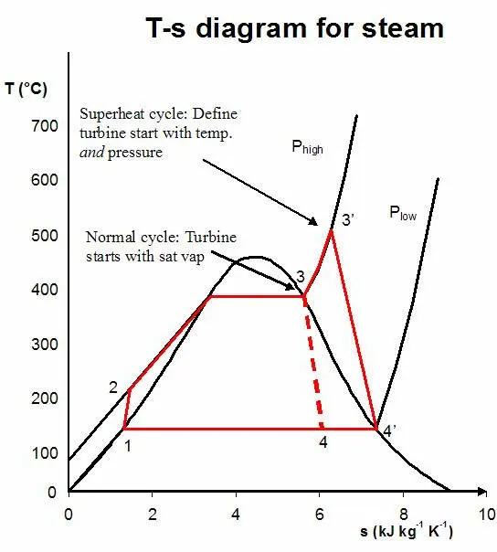
Rankine engines generally operate in a closed loop where the working fluid is reused. The water vapor with condensed droplets often seen billowing from power stations is created by the cooling systems (not directly from the closed-loop Rankine power cycle). This 'exhaust' heat is represented by the "Qout" flowing out of the lower side of the cycle shown in the T–s diagram below. Cooling towers operate as large heat exchangers by absorbing the latent heat of vaporization of the working fluid and simultaneously evaporating cooling water to the atmosphere.
There are four processes in the Rankine cycle. The states are identified by numbers (in brown) in the T–s diagram.
- Process 1–2: The working fluid is pumped from low to high pressure. As the fluid is a liquid at this stage, the pump requires little input energy. Process 1-2 is isentropic compression.
- Process 2–3: The high-pressure liquid enters a boiler, where it is heated at constant pressure by an external heat source to become a dry saturated vapour. The input energy required can be easily calculated graphically, using an enthalpy–entropy chart (h–s chart, or Mollier diagram), or numerically, using steam tables or software. Process 2-3 is constant pressure heat addition in boiler.
- Process 3–4: The dry saturated vapour expands through a turbine, generating power. This decreases the temperature and pressure of the vapour, and some condensation may occur. The output in this process can be easily calculated using the chart or tables noted above. Process 3-4 is isentropic expansion.
- Process 4–1: The wet vapour then enters a condenser, where it is condensed at a constant pressure to become a saturated liquid. Process 4-1 is constant pressure heat rejection in condenser.
In an ideal Rankine cycle the pump and turbine would be isentropic, i.e., the pump and turbine would generate no entropy and hence maximize the net work output. Processes 1–2 and 3–4 would be represented by vertical lines on the T–s diagram and more closely resemble that of the Carnot cycle. The Rankine cycle shown here prevents the state of the working fluid from ending up in the superheated vapor region after the expansion in the turbine, [1] which reduces the energy removed by the condensers.
RESULT OF SUMILATOR:
Procedure:
- Starting the program with close all and clc
- By using disp command writing the header for result in simulator, the four process of
- Isentropic expansion (turbine)
- Constant pressure heat rejection in (conducer)
- Isentropic compression (pump)
- Constant pressure heat addition (boiler)
- By using input command considering the values of ‘p1, t1, p2’ those displayed at command window for assigning numerical values.
- Calculation values of p, t, h, s pressures, temperature, enthalpy, entropy this will be followed in every four stages.
- Stage -1 the steam with constant pressure is expands in turbine so the p1 t1 are already given, the enthalpy and entropy values are extracted from the file Xsteam where pre-loaded steam tables this is followed in every stage.
- Stage -2 the expanded steam at low pressure converted to water and conduce down at conducer where the heat is rejected. Hear the entropy is same so s1=s2.
By using dryness fraction deriving the enthalpy h2.
The process from 1-2 the gas(vapour) is converting to liquid(fluid) so extracting specific enthalpy and specific entropy at p2 for both gas and liquid.
- Stage-3 the condensed liquid travels to pump, then the pressure p3=p2 and t3=t2. the pressure is low so the enthalpy and entropy h, s at low pressure extracted from Xsteam file.
- Stage -4 the liquid at low pressure is converted into high pressure by the mean of pump so p4=p1. and the liquid travels to boiler and the temperature raises to t4 than the liquids is converted to vapour
The constant pressure cp and constant volume cv are extracted and the gamma value is calculated and by this t4 temperature is calculated. Entropy will be same.
- The temperature at two more stages is calculated t5, t6 for feasibility of plotting.
- At last calculating efficiency parameters
- work down by pump
wp=v3*(p4-p3) *1000
h4=h3+wp;
- Work down by turbine
wt=h1-h2;
- net work done
wnet=wt-wp;
- heat supplyed
q_in=h1-h4;
q_out=h2-h3;
- thermal efficiency
Nthermo=wnet/q_in;
- steam conductivity
steam_rate=3600/(wt-wp);
- back work ratio
bwr=wp/wt;
- plotting:
dividing the single window to 2 and making 2 plots by the command subplot (1,2,1)
plotting T-S plot taking temperature as a array and by using for loop to cycle reaction.
By using plot commend and plotting T and s points at 4 stages.
By using text commend marking direction of change in process due to t and s.
By using label commend setting the axis
- Plotting
Taking subplot as (1,2,2)
By plot command plotting all the points of s h at every 4 stages.
By text command plotting the direction
By using label commend setting the axis
RESULT:
The Rankine cycle plots have generated by calculating the state points, efficiency and the output is printed in the command window.
Plots in the screen shots.
CONCLUSION:
The values of all state points of pressure temperature enthalpy entropy and work done efficiency are calculated and plotted.
These parameters are changes in different power plants according to the equipment installed and arrangement.
The rankin cycle exist simulated according to the values given.