Project 2 - Rankine cycle Simulator
AIM
Create a Rankine Cycle Simulator using MATLAB.
OBJECTIVE
- Create a code to calculate the state points of the Rankine Cycle (any type of your choice) based on user inputs.
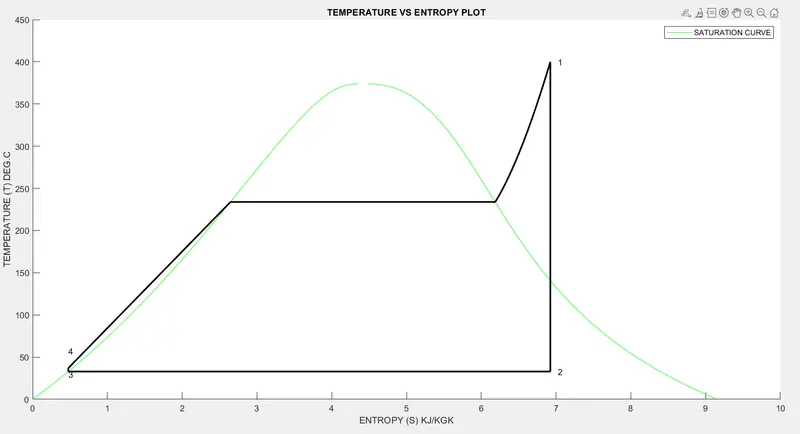
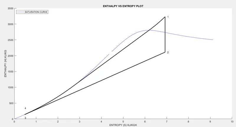
- plot the corresponding T-s and h-s plots for the given set of inputs.
RANKINE CYCLE
Rankine Cycle is a mechanical cycle commonly used in power plant to convert the pressure energy of steam into mechanical energy through steam turbines. The Rankine Cycle’s major components include a rotating steam turbine, a boiler pump, a stationary condenser, and a boiler.
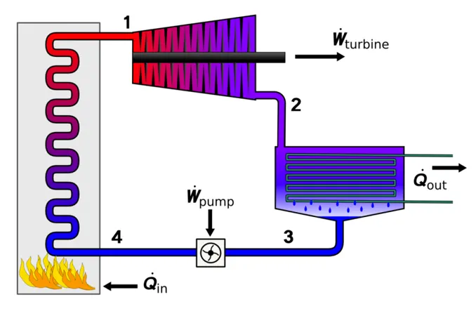
Process 1-2 is isentropic expansion in turbine
The dry saturated vapour comming from the boiler expands through a turbine, generating power. This decreases the temperature and pressure of the vapour, and some condensation may occur. The output in this process can be easily calculated using the chart or tables or software
Process 2-3 is constant pressure heat rejection in condenser
The wet vapour then enters a condenser, where it is condensed at a constant pressure to become a saturated liquid.
Process 3-4: is isentropic compression
The working fluid is pumped from low to high pressure. As the fluid is a liquid at this stage, the pump requires little input energy.
Process 4-1 is constant pressure heat addition in boiler
The high-pressure liquid enters a boiler, where it is heated at constant pressure by an external heat source to become a dry saturated vapour. The high-pressure liquid enters a boiler, where it is heated at constant pressure by an external heat source to become a dry saturated vapour. The input energy required can be easily calculated graphically, using an enthalpy-entropy chart(h-s chart, or mollier diagram), or numerically, using steam table or software.
MATLAB CODE
clear all
close all
clc
disp('RANKINE CYCLE');
disp('process 1-2  isentropic expoansion in turbine')
disp('process 2-3 constant pressure heat rejection in condenser')
disp('process 3-4 isentropic compression in pump')
disp('process 4-1 consant pressure heat addition in boiler')
% accepting input from user
T1=input('enter the turbine inlet temp,t1 (in deg.c)=');
p1=input('enter the turbine inlet pressure,p1 (in bar)=');
p2=input('enter the turbine outlet pressure,p2 (in bar)=');
% getting data from xsteam file and defining values

%state 1
h1=XSteam('h_pT',p1,T1);
s1=XSteam('s_pT',p1,T1);

%state 2
s2=s1 ;
sf2=XSteam('sL_p',p2);
sg2=XSteam('sV_p',p2);
x2=(s2-sf2)/(sg2-sf2);
hf2=XSteam('hL_p',p2);
hg2=XSteam('hV_p',p2);
h2=hf2+(x2*(hg2-hf2));

%state 3
p3=p2;
s3=XSteam('sL_p',p3);
h3=XSteam('hL_p',p3);

%state 4
s4=s3;
p4=p1;

%work done by turbine
wt= h1-h2;
%work done by pump
v3=XSteam('vL_p',p3);
wp=v3*(p4-p3)*100;

%pump work=h4-h3, therefore
h4=h3+wp;

%net work done
wnet=wt-wp;

% calculating thermal efficency
qin=h1-h4; % heat in
qout=h2-h3; %heat out
therm_eff= (wnet/qin)*100;

%specific steam consumption  Specific Steam Consumption or Steam Rate (SSC)
% is the mass flow rate of steam required to produce 1 kW net work output
ssc=(3600/wnet);

%determining temperature at remaining state points
T3=XSteam('Tsat_p', p3);
T2=T3;
cp4=XSteam('Cp_ps',p4,s4);
cv4=XSteam('Cv_ps',p4,s4);
k=cp4/cv4;
T4=T3/((p3/p4)^((k-1)/k));

%At vapour and liquid line
T6=XSteam('Tsat_P',p1);
s5=XSteam('sL_p',p1);
s6=XSteam('sV_p',p1);
h5=XSteam('hL_p',p1);
h6=XSteam('hV_p',p1);
T5=T6;

% plotting the saturation curve
T=linspace(1,375,1000);
for i= 1:length(T)
    sf(i)=XSteam('sL_T', T(i));
    sg(i)=XSteam('sV_T', T(i));
    hf(i)=XSteam('hL_T', T(i));
    hg(i)=XSteam('hV_T', T(i));
end

%plotting T-S diagram
figure(1)
hold on
plot(sf,T,'color','g')
plot(sg,T,'color','g')

plot([s1 s2],[T1,T2],'k','linewidth',2)
plot([s2 s3],[T2 T3,],'k','linewidth',2)
plot([s3 s4],[T3 T4,],'k','linewidth',2)
plot([s4 s5],[T4 T5,],'k','linewidth',2)
plot([s5 s6],[T5 T6,],'k','linewidth',2)
sc1=linspace(s6,s1,1000);
for i=1:length(sc1)
    Tc1(i)= XSteam('T_ps',p1,sc1(i));
end
plot(sc1,Tc1,'k','LineWidth',2)
text(s1+0.1,T1,'1')
text(s2+0.1,T2,'2')
text(s3,p1,T3-20,'3')
text(s4,T4+20,'4')
title('TEMPERATURE VS ENTROPY PLOT')
xlabel('ENTROPY (S) KJ/KGK')
ylabel('TEMPERATURE (T) DEG.C')
legend('SATURATION CURVE')

%plotting H-S diagram
figure(2)
hold on
plot(sf,hf,'color','b')
plot(sg,hg,'color','b')
plot([s1 s2],[h1 h2],'k','LineWidth',2)
plot([s2 s3],[h2 h3],'k','linewidth',2)
plot([s3 s4],[h3 h4],'k','linewidth',2)
hc= linspace(h4,h5,100);
for j=1:length(hc)
    sch(j)=XSteam('s_ph',p1,hc(j));
end
plot(sch,hc,'k','LineWidth',2)
plot([s5 s6],[h5 h6],'k','LineWidth',2)
for k=1:length(sc1)
hc1(k)=XSteam('h_ps',p1,sc1(k));
end
plot(sc1,hc1,'k','LineWidth',2)
text(s1+0.1,h1,'1')
text(s2+0.1,h2,'2')
text(s3,h3-100,'3')
text(s4,h4+200,'4')
title('ENTHALPY VS ENTROPY PLOT')
xlabel('ENTROPY (S) KJ/KGK')
ylabel('ENTHALPY (H) KJ/KG')
legend('SATURATION CURVE','Location','northwest')
% Displaying Results
disp(' DISPLAYING RESULTS');
fprintf('At State Point 1 \n');
fprintf('p1: %8.3f bar \n', p1);
fprintf('T1: %8.3f C \n', T1);
fprintf('h1: %8.3f KJ/kg \n', h1);
fprintf('s1: %8.3f KJ/kgK \n', s1);
fprintf('At State Point 2 \n');
fprintf('p2: %8.3f bar \n', p2);
fprintf('T2: %8.3f C \n', T2);
fprintf('h2: %8.3f kJ/kg \n', h2);
fprintf('s2: %8.3f kJ/kgK \n', s2);
fprintf('x2: %8.3f \n', x2);
fprintf('At State Point 3 \n');
fprintf('p3: %8.3f bar \n', p3);
fprintf('T3: %8.3f K \n', T3);
fprintf('h3: %8.3f kJ/kg \n', h3);
fprintf('s3: %8.3f kJ/kgK \n', s3);
fprintf('At State Point 4 \n');
fprintf('p4: %8.3f  /', p4);
fprintf('T4: %8.3f K \n', T4);
fprintf('h4: %8.3f KJ/kg \n', h4);
fprintf('s4: %8.3f kJ/kgK \n', s4);
fprintf('Turbine Work: %8.3f kJ/kg \n', wt);
fprintf('Pump Work: %8.3f kJ/kg \n', wp);
fprintf('Wnet: %8.3f kJ/kg \n', wnet);
fprintf('Efficiency: %8.3f Percent \n ', therm_eff);
fprintf('SSC: %8.3f kJ/kWh', ssc);
CODE EXPLANATION
XSteam data usage is simmilar to steam table usage in thermal engineering. Here we extract liquid and gaseous properties of enthalpy, and entropy at specific pressure and temperature for saturated liquid and saturated vapour conditions.
The 4 states are displayed the user and the user is asked to enter turbine inlet temperature, turbine inlet and outle pressure.
with the above available data, proper eqautions and xsteam data we are able to compute values for all state point.
eg: Using XSteam.dat file the command h1=XSteam('h_pT', p1,T1) and s1=XSteam('s_pT',p1,T1) will return values for enthalpy and entropy at point 1, simmilarly we find other values.
In case of sf, sg, hf, hg the f (fluid) and g stands for saturated liquid and saturated vapour. Using appropriate equations net work done, thermal efficency and SSC(specific steam consumption) are calculated. T,S and H values are extracted at vapour and liquid line.
Plotting is done for T VS H and H vs S
Other than the state points a saturation line is also plotted (for saturated liquid and saturated vapour) and identified in the graph using 'legend' command.
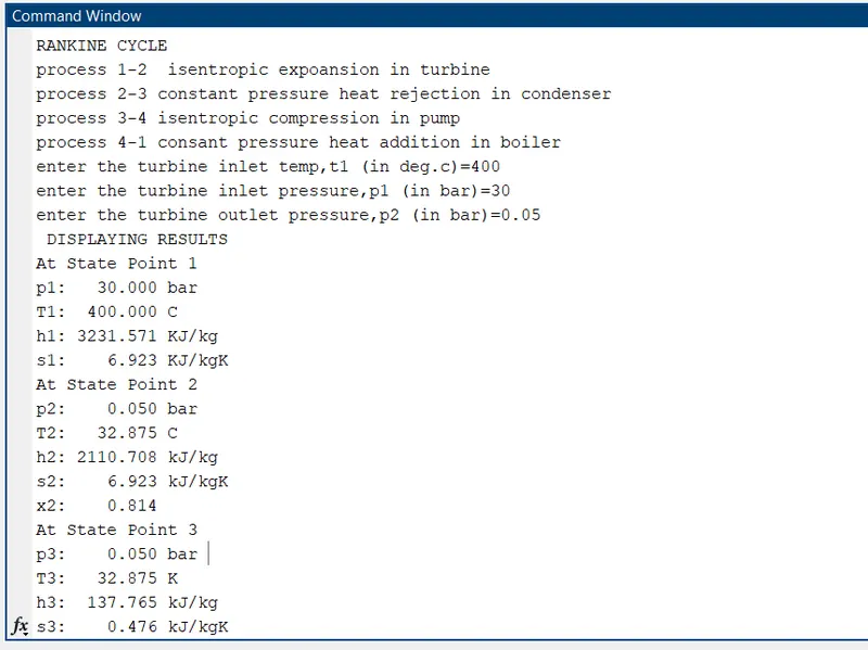
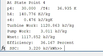
We will get different results based on user input and the results are displayed in command window.
OUTPUTS
1)TEMPERATURE VS ENTROPY PLOT
2) ENTHALPY VS ENTROPY PLOT
3) COMMAND WINDOW
CONCLUSION
- Created a rankine cycle simulator using matlab and obtained the results
- All the results are satisfactory
REFERENCE