Project 2 - Rankine cycle Simulator

PROGRAM :

clear all
close all
clc

% Printing Introduction
fprintf('RANKINE CYCLE SIMULATOR \n')
fprintf('\n1-2 is isentropic expantion in the turbine \n')
fprintf('2-3 is constant pressure heat rejection by the condencer \n')
fprintf('3-4 is isentropic compression in pump \n')
fprintf('4-1 is constant pressure heat Addition by the boiler \n')

% Inputs
P1 = 30; %('\nEnter the pressure at the turbine Inlet (in bar): ');
T1 = 400;%('Enter the temperature at the turbine Inlet (in Degree celcius): ');
P2 = 5;  %('Enter the pressure at the turbine Outlet (in bar): ');

% state point 1
H1 = XSteam('h_pt',P1,T1);   %Enthalpy
S1 = XSteam('s_pt',P1,T1);   %Entropy
Hf1 = XSteam('hL_p',P1);     %Enthalpy of saturated liquid
Hg1 = XSteam('hV_p',P1);     %Enthalpy of saturated vapour
Ts1 = XSteam('Tsat_p',P1);   %saturation Temperature
Sf1 = XSteam('sL_p',P1);     %Entropy of saturated liquid
Sg1 = XSteam('sV_p',P1);     %Entropy of saturated vapour

% state point 2
S2 = S1;
Sf2 = XSteam('sL_p',P2);
Sg2 = XSteam('sV_p',P2);
X = (S2-Sf2)/(Sg2-Sf2);     % Dryness Fraction
Hf2 = XSteam('hL_p',P2);
Hg2 = XSteam('hV_p',P2);
H2 = Hf2 + X*(Hg2-Hf2);
T2 = XSteam('T_ph',P2,H2);
Ts2 = XSteam('Tsat_p',P2);

% state point 3
H3 = Hf2;
S3 = Sf2;
T3 = T2;
P3 =  P2;

% state point 4
P4 = P1;
S4 = S3;
H4 = XSteam('h_ps',P4,S4);
T4 = XSteam('T_ps',P4,S4);

t = linspace(0,374,500);    % temp space for plotting saturation cutves

% plot T-S Diagram
figure(1)
hold on

% plot saturation curve
for i = 1:length(t)
    plot(XSteam('sL_T',t(i)),t(i),'.','Color','b')
    plot(XSteam('sV_T',t(i)),t(i),'.','Color','b')
end

% plot Cycle
plot([S1 S2],[T1 T2],'linewidth',2,'Color','r')
if X>1
    T3 = Ts2;
    plot([S2 Sg2 S3 S4],[T2 Ts2 T3 T4],'linewidth',2,'Color','r')
    T2 = Ts2;
else
   plot([S2 S3 S4],[T2 T3 T4],'linewidth',2,'Color','r')
end
l = linspace(T1,T2,1000);
for i = 1:length(l)
    plot(XSteam('s_pT',P1,l(i)),l(i),'.','Color','r')
end
plot([Sf1 Sg1],[Ts1 Ts1],'linewidth',2,'Color','r')
xlabel('Enthalpy[KJ/Kg-K]')
ylabel('Temperature[K]')
title('T-S Diagram')


%plot H-S Diagram
figure(2)
hold on
%plot saturation curve
for i = 1:length(t)
    plot(XSteam('sL_T',t(i)),XSteam('hL_T',t(i)),'.','color','b')
    plot(XSteam('sV_T',t(i)),XSteam('hV_T',t(i)),'.','color','b')
end
%plot Cycle
plot([S1 S2 S3 S4 S1],[H1 H2 H3 H4 H1],'linewidth',2,'Color','r')
xlabel('Entropy[KJ/Kg-K]')
ylabel('Enthalpy[KJ/Kg]')
title('H-S Diagram')

% Calculations

% Turbine Work
Wt = H1-H2;
% Pump work
Wp = H4-H3;
% Heat Addition
Qin = H1-H4;
% Heat rejection
Qout = H2-H3;
% Net work
Wnet = Wt-Wp;
% Efficiency
Ntherm = (Wnet/Qin)*100;
% Specific steam consumption
SSC = 3600/Wnet;
% Back work Ratio
BWR = Wp/Wt;

% Print Results
fprintf('\n\nResults\n')
fprintf('At state point 1:\n')
fprintf('P1 is : %.2f bar\n',P1)
fprintf('T1 is : %.2f Deg celcius\n',T1)
fprintf('H1 is : %.2f KJ/Kg\n',H1)
fprintf('S1 is : %.2f KJ/Kg\n',S1)

fprintf('At state point 2:\n')
fprintf('P2 is : %.2f bar\n',P2)
fprintf('T2 is : %.2f Deg celcius\n',T2)
fprintf('H2 is : %.2f KJ/Kg\n',H2)
fprintf('S2 is : %.2f KJ/Kg\n',S2)

fprintf('At state point 3:\n')
fprintf('P3 is : %.2f bar\n',P3)
fprintf('T3 is : %.2f Deg celcius\n',T3)
fprintf('H3 is : %.2f KJ/Kg\n',H3)
fprintf('S3 is : %.2f KJ/Kg\n',S3)

fprintf('At state point 4:\n')
fprintf('P4 is : %.2f bar\n',P4)
fprintf('T4 is : %.2f Deg celcius\n',T4)
fprintf('H4 is : %.2f KJ/Kg\n',H4)
fprintf('S4 is : %.2f KJ/Kg\n',S4)

fprintf('\nWt is : %.2f KJ/Kg\n',Wt)
fprintf('Wp is : %.2f KJ/Kg\n',Wp)
fprintf('Wnet is : %.2f KJ/Kg\n',Wnet)
fprintf('ThermalEfficiancy is : %.2f percent\n',Ntherm)
fprintf('S.S.C. is : %.2f Kg/KWh\n',SSC)
fprintf('Back work Ratio is : %.3f \n',BWR)

AIM :

To simulate the Rankine Cycle and plot the corresponding T-S and H-S plots using MATLAB.

OBJECTIVES :

Calculate the state points of the Rankine Cycle based on given inputs.

plot the corresponding T-S and H-S plots for the given set oututs.

GIVEN:

INPUT VALUES:

Turbine inlet temperare = 400'C

Turbine inlet Pressure = 30 bars

Turbine Outlet pressure = 0.05 bars = Condencer Inlet pressure

REQUIRED OUTPUT VALUES:

Net Work Output

Back Work Rtio

RANKINE CYCLE SIMULATOR:

Rankine Cycle converts thermal energy to mechanical energy.

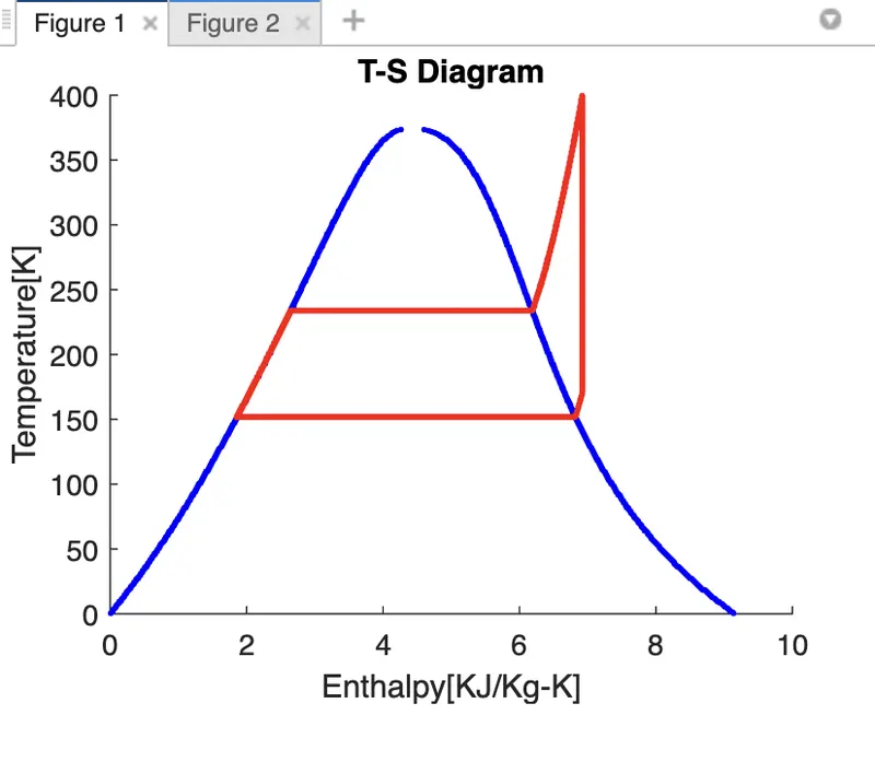
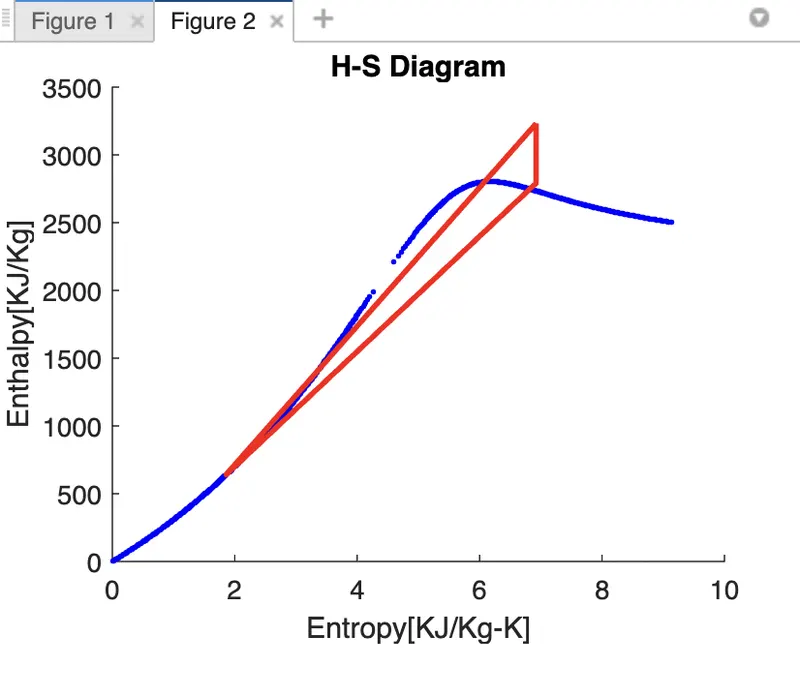
The Ideal Rankine Cycle consists of the following processes:

1-2 is Isentropic expantion of the turbine.

2-3 is constant pressure Heat rejection by the condencer.

3-4 is Isentropic compression in pump.

4-1 is constant pressure Heat addition by the boiler.

First all the requird variables and parameters were found out to calculate.

Then using the XSteam library function ,all the parameters were sorted out.

Then the usual calculation and plotting of the graphs were done as per the therory of thermodynamics.

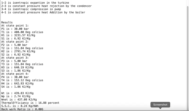
COMMAND WINDOW :

T-S PLOTS :

H-S PLOTS :

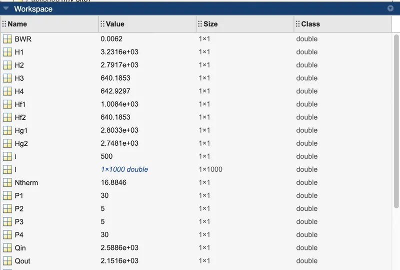
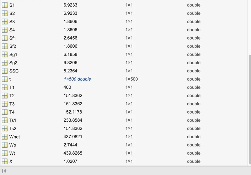
WORKSPACE VALUES :

ERRORS:

No complicated errors occurred while running the MATLAB program.

CONCLUTION :

The required output values are obtained for the given input parameters:

Net Work Outpt = 437.08 KJ/Kg

Back Work Ratio = 0.006

Thus the Rankine cycle is successfully simulated by using MATLAB.