Project 2 - Rankine cycle Simulator
AIM:- To create Rankine cycle simulation
THEORY:- The Rankine cycle in a model used to predict the performance of a steam turbine It is also used to predict the performance ofthe reciprocating steam engine . The rankine cycle is the idealized thermodynamic cycle of the heat engine that converted heat to mechanical work The Rankine cycle closely describes the process by which steam engines commonly found in thermal power generation plant hearn the he thermal energy of a fuel or other heat source to generate electricity. Possible heat sources include combustion of fossil fuels such as coal, natural gas, or oil, renewable fuels like biomass or ethanol and Common heat sinks include ambient air above or around a facility and bodies of water such as rivers, ponds, and oceans.
The Rankine cycle or Rankine Vapor Cycle is the process widely used by power plants such as coal-fired power plants or nuclear reactors. In this mechanism, a fuel is used to produce heat within a boiler, converting water into steam which then expands through a turbine producing useful work. This process was developed in 1859 by Scottish engineer William J.M. Rankine.
Processes of Rankine Cycle :
The ideal Rankine cycle consists of the following four processes:
1-2 Isentropic expansion in a turbine
2-3 Constant pressure heat rejection in a condenser
3-4 Isentropic work addition in a pump
4-1 Constant pressure heat addition in a boiler
In figure Schematic representation of an ideal Rankine cycle is shown.
Figure : Schematic representation of an ideal Rankine cycle
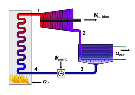
Figure: T-s diagram of an ideal Rankine cycle
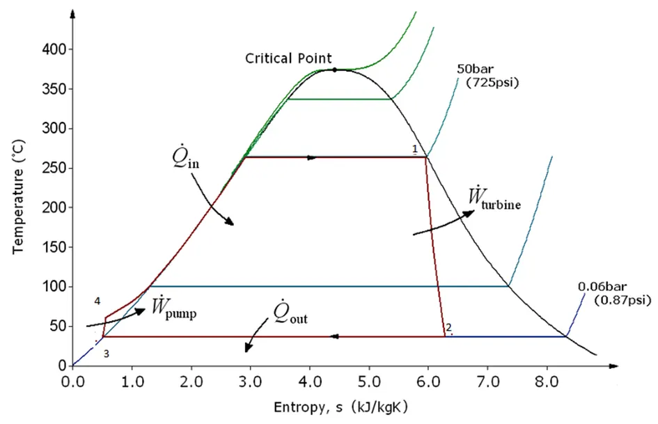
There are four processes in the Rankine cycle. The states are identified by numbers in the T–s diagram.
• Process 1–2: The dry saturated vapour expands through a turbine, generating power. This decreases the temperature and pressure of the vapour, and some condensation may occur. In other words Process 1-2 is [Isentropic expansion]
• Process 2–3: The wet vapour then enters a condenser, where it is condensed at a constant pressure to become a saturated liquid. In other words Process 2-3 is [Constant pressure heat rejection in condenser]
• Process 3–4: The working fluid is pumped from low to high pressure. As the fluid is a liquid at this stage, the pump requires little input energy. In other words Process 3-4 is [Isentropic compression]
• Process 4–1: The high-pressure liquid enters a boiler, where it is heated at constant pressure by an external heat source to become a dry saturated vapour. The input energy required can be easily calculated graphically, using an enthalpy–entropy chart (h–s chart, or Mollier diagram), or numerically, using steam tables. In other words Process 4-1 is [Constant pressure heat addition in boiler]
In an ideal Rankine cycle the pump and turbine would be isentropic, i.e., the pump and turbine would generate no entropy and hence maximize the net work output.
Calculatations
Work done on pump, per kg of water
WP=h4−h3WP=h4-h3
Energy added in steam generator,
qin=h1−h4qin=h1-h4
Work delivered by turbine,
WT=h1−h2WT=h1-h2
Energy rejected in the condenser, qout=h2−h3qout=h2-h3
Net work output, Wnet=WT−WPWnet=WT-WP
Back work ratio : Ratio of Pump work required and Turbine work generated.
The thermal efficiency of the Rankine cycle is given by,
η=Wnetqin=WT−WPqinη=Wnetqin=WT-WPqin
η=(h1−h2)−(h4−h3)(h1−h4)η=(h1-h2)-(h4-h3)(h1-h4)
η=(h1−h4)−(h2−h3)(h1−h4)=1−(h2−h3)(h1−h4)η=(h1-h4)-(h2-h3)(h1-h4)=1-(h2-h3)(h1-h4)
By this equation efficiency of Rankine cycle is calculated.
% project of rankine cycle
clear all
close all
clc

%print heading
fprintf('n                        RANKIN CYCLE SIMULATION');
fprintf('\n n1-2            is isentropic expantion in the Turbine');
fprintf('\n n2-3                is constant pressurre heat rejection');


%input perameter
p1 = 30 %Enter Turnine Inlet pressure(in bar)
T1 = 400 %Enter turbine inlet temparature(in k )
p2 = 0.05 %Enter the pressurea at condensure(inbar)

%calculating various perameter in rankine cycle
%h represent enthalpy
%s represent entropy
%T represent temparature
%P represent pessure
%v reoresent valeum


%for state point one
h1 = XSteam('h_pt',p1,T1);
s1 = XSteam('s_pt',p1,T1);

%for state point 3
p3 = p2;
h3 = XSteam('hL_p',p3);
s3 = XSteam('sL_p',p3);
v3 = XSteam('vL_p',p3);
t3 = XSteam('Tsat_p',p3);

%for state point
t2 = t3'
s2 = s1;
sf2 = XSteam('sL_p',p2);
sg2 = XSteam('sV_p',p2);
hf2 = XSteam('hL_p',p2);
hg2 = XSteam('hV_p',p2);
x2 = ((s2-sf2)/(sg2-sf2));
h2 = hf2+(x2*(hg2-hf2));

%for state point 4
p4 = p1;
s4 = s3;
cp4 = XSteam('Cp_ps',p4,s4);
cv4 = XSteam('Cv_ps',p4,s4);
g4 = cp4/cv4;
o = (g4-1)/g4;
t4 = t3*((p4/p3)^o);

%pump work
Wp = v3*(p4-p3)*100
%wp = h4/h3 from this calculation
h4  = h3+Wp;

%turbine work
Wt = h1-h2

%Net work
Wnet  = Wt-Wp
%heat addition at steam generation
Qin = h1 - h4;
%heat rejection at condesear
Qout = h2 - h4;

%thermal efficiency of cycle
Ntherm  = (Wnet/Qin)*100;

%bck work ratio: ratio of pump work required and turbine work generator
BWR = Wp/Wt

%calculation value of liquied and vepour satureted line
pressure_range = 0:0.1:100;
for i = 1:length(pressure_range)
    tL_sat(i) = XSteam('Tsat_p',pressure_range(i));
    sL_sat(i) = XSteam('sL_p',pressure_range(i));
    sV_sat(i) = XSteam('sV_p',pressure_range(i));
    hL_sat(i) = XSteam('hL_p',pressure_range(i));
    hV_sat(i) = XSteam('hV_p',pressure_range(i));
end
%ploting graph for state 4 and 1 on T and S values
tp = XSteam('tsat_p',p4); %temparature between satureted liquied and saturede vepour line
s4_L = XSteam('sL_T',tp);
s4_V = XSteam('sV_T',tp);

t_range = linspace(tp,T1,400);
for i = 1:length(t_range);
    s4V_1(i) = XSteam('s_pT',p4,t_range(i));
end

%ploting the results
%difiend figure propertys
figure('units','normalized','outerposition',[0 0 1 1])

figure(1)

%copleted resukts using subpolt
ax = subplot(6,4,[1,2,3,4,5,6,7,8]);
text(0.4,1,'RANKINE CYCLE SIMULATION','fontsize',12,'fontweight','bold')
text(0,0.8,'1-2 Isentropic Expostion in Turbine');
text(0,0.7,'2-3 is constsnt pressure heat rejection by the condeser')
text(0,0.6,'3-4 is insentropic comprestion in pump');
text(0,0.5,'4-1 is constant pressure heat addition');
text(0,0.3,['Enter Turnine Inlet pressure(in bar) : ' ,num2str(p1)]);
text(0,0.2,['Enter turbine inlet temparature(in k ) : ',num2str(T1)]);
text(0,0.1,['Enter the pressurea at condensure(inbar) : ',num2str(p2)]);
text(0.47,0,'RESULT','fontweight','bold');


set(ax,'visible','off')

%print stage 1 values
ax = subplot(6,4,[9,13]);
text(0,1,'at state point 1 : ');
text(0,0.8,['p1 is : ',num2str(p1),'Bar']);
text(0,0.7,['T1 is : ',num2str(T1),'gedree']);
text(0,0.6,['h1 is : ',num2str(h1),'kj/kg']);
text(0,0.5,['S1 is : ',num2str(s1),'kj/kgk']);
set(ax,'visible','off')

%print work done efficiency
text(0,0.3,'other results : ');
text(0,0.2,['Wt is : ',num2str(Wt),'kj/kg']);
text(0,0.1,['Wp is : ',num2str(Wp),'kj/kg']);
text(0,0,['Wnet is : ',num2str(Wnet),'kj/kg']);
set(ax,'visible','off')

%print stage 2
 ax =  subplot(6,4,[10,14]);
 text(0,1,'at state point 2 : ');
text(0,0.8,['p2 is : ',num2str(p2),'Bar']);
text(0,0.7,['t2 is : ',num2str(t2),'gedree']);
text(0,0.6,['h2 is : ',num2str(h2),'kj/kg']);
text(0,0.5,['s2 is : ',num2str(s2),'kj/kgk']);
text(0,0.2,['BWR is : ',num2str(BWR)]);
text(0,0.1,['Ntherm is : ',num2str(Ntherm)]);

set(ax,'visible','off')

%print state 3 values
ax = subplot(6,4,[11,15]);
text(0,1,'at state point 3 : ');
text(0,0.8,['p3 is : ',num2str(p3),'Bar']);
text(0,0.7,['t3 is : ',num2str(t3),'gedree']);
text(0,0.6,['h3 is : ',num2str(h3),'kj/kg']);
text(0,0.5,['s3 is : ',num2str(s3),'kj/kgk']);
set(ax,'visible','off')


%print state 4 values
ax = subplot(6,4,[12,16]);
text(0,1,'at state point 4 : ');
text(0,0.8,['p4 is : ',num2str(p4),'Bar']);
text(0,0.7,['t4 is : ',num2str(t4),'gedree']);
text(0,0.6,['h4 is : ',num2str(h4),'kj/kg']);
text(0,0.5,['s4 is : ',num2str(s4),'kj/kgk']);
set(ax,'visible','off')

%ploting T S daigream using subplot
subplot(6,4,[17,18,21,22]);
hold on
plot(sL_sat,tL_sat,'linestyle','--','linewidth',1,'color','b')
plot(sV_sat,tL_sat,'linestyle','--','linewidth',1,'color','b')
plot([s1 s2 s3 s4 s4_L s4_V s4V_1],[T1 t2 t3 t4 tp tp t_range],'linewidth',1.5,'color','r')
title('T-S diagram of rankine cycle')
xlabel('Enthalpy')
ylabel('Temperature')

%plot H-S diagram using subplot
subplot(6,4,[19,20,23,24])
hold on
plot(sL_sat,hL_sat,'Linestyle','--','linewidth',1,'color','b')
plot(sV_sat,hV_sat,'Linestyle','--','linewidth',1,'color','b')
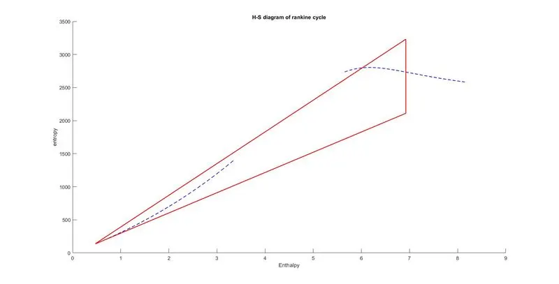
plot([s1 s2],[h1 h2],'linewidth',1.5,'color','r')
plot([s2 s3],[h2 h3],'linewidth',1.5,'color','r')
plot([s3 s4],[h3 h4],'linewidth',1.5,'color','r')
plot([s4 s1],[h4 h1],'linewidth',1.5,'color','r')
title('H-S diagram of rankine cycle')
xlabel('Enthalpy')
ylabel('entropy')

%creating second figure which is individual show TS daigram

figure('units','normalized','outerposition',[0 0 1 1])
figure(2)
hold on
plot(sL_sat,tL_sat,'Linestyle','--','linewidth',1,'color','b')
plot(sV_sat,tL_sat,'Linestyle','--','linewidth',1,'color','b')
plot([s1 s2 s3 s4 s4_L s4_V s4V_1],[T1 t2 t3 t4 tp tp t_range],'linewidth',1.5,'color','r')
title('T-S diagram of rankine cycle')
xlabel('Enthalpy')
ylabel('Temperature')

%creating 3rd figure which is individual show H - S Diagram
figure('units','normalized','outerposition',[0 0 1 1])
figure(3)
hold on
plot(sL_sat,hL_sat,'Linestyle','--','linewidth',1,'color','b')
plot(sV_sat,hV_sat,'Linestyle','--','linewidth',1,'color','b')
plot([s1 s2],[h1 h2],'linewidth',1.5,'color','r')
plot([s2 s3],[h2 h3],'linewidth',1.5,'color','r')
plot([s3 s4],[h3 h4],'linewidth',1.5,'color','r')
plot([s4 s1],[h4 h1],'linewidth',1.5,'color','r')
title('H-S diagram of rankine cycle')
xlabel('Enthalpy')
ylabel('entropy')
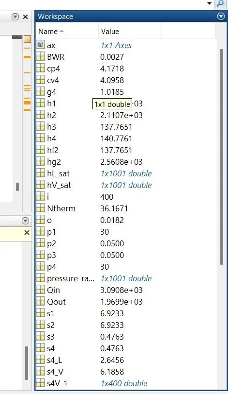
Figure 1 : Complete Result
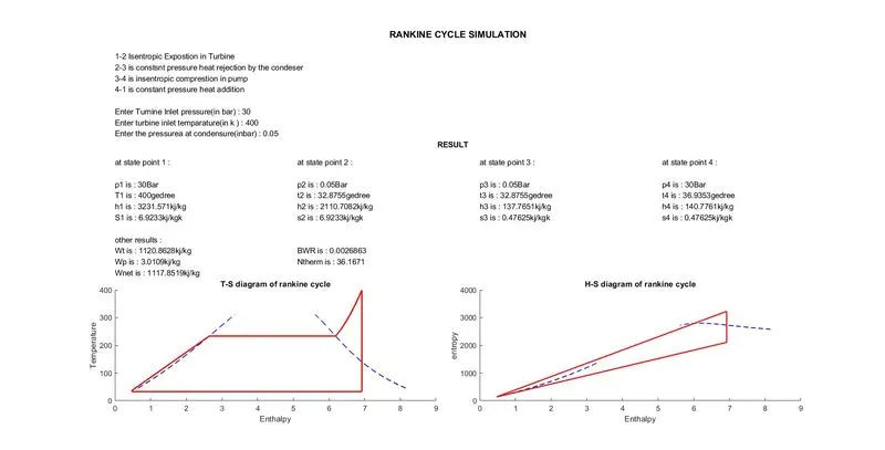
Figure 2 : T-S Diagram
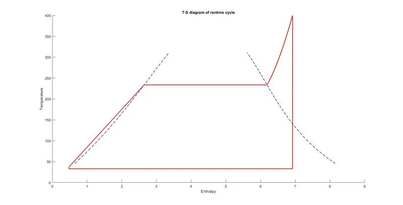
Figure 3 : H-S Diagram
ERROR