Project 2 - Rankine cycle Simulator

Aim: To create a Rankine Cycle Simulator using OCTAVE/MATLAB.

Objective:

• To calculate the state points of the Rankine Cycle.
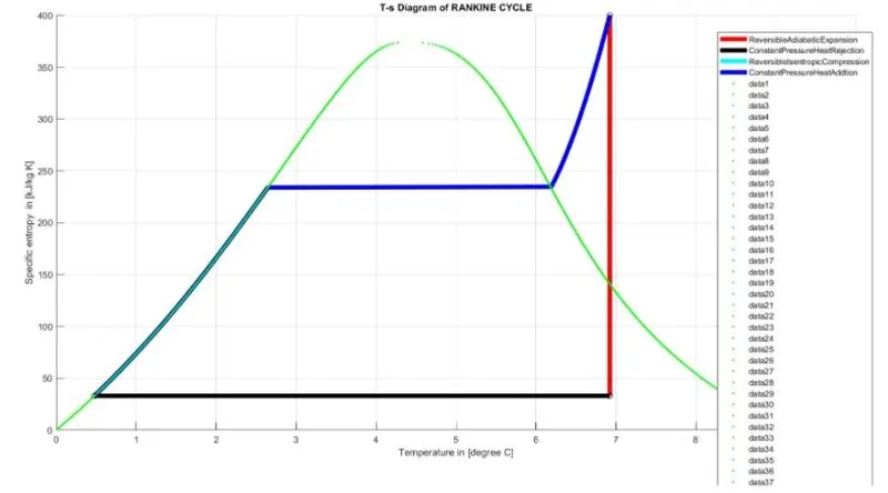
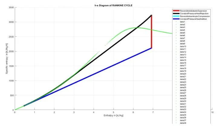
• Plot the corresponding T-s and h-s plots for the given set of inputs.

Theory: The Rankine cycle is an idealized thermodynamic cycle describing the process by which certain heat engines, such as steam turbines or reciprocating steam engines, allow mechanical work to be extracted from a fluid as it moves between a heat source and heat sink. The Rankine cycle is named after William John Macquorn Rankine, a Scottish polymath professor at Glasgow University.

The Rankine cycle closely describes the process by which steam engines commonly found in thermal power generation plants harness the thermal energy of a fuel or other heat source to generate electricity. Possible heat sources include the combustion of fossil fuels such as coal, natural gas, or oil, renewable fuels like biomass or ethanol, nuclear fission, and concentrated solar power. Common heat sinks include ambient air above or around a facility and bodies of water such as rivers, ponds, and oceans.

The ability of a Rankine engine to harness energy depends on the relative temperature difference between the heat source and heat sink. The greater the differential, the more mechanical power can be efficiently extracted out of heat energy, as per Carnot's theorem.

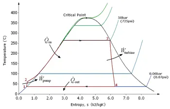
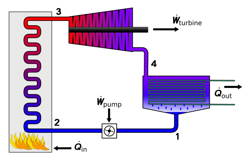
There are four processes in the Rankine cycle. The states are identified by numbers (in brown) in the T–s diagram.

• Process 1–2: The working fluid is pumped from low to high pressure. As the fluid is a liquid at this stage, the pump requires little input energy. Process 1-2 is isentropic compression.
• Process 2–3: The high-pressure liquid enters a boiler, where it is heated at constant pressure by an external heat source to become a dry saturated vapour. The input energy required can be easily calculated graphically, using an enthalpy–entropy chart (h–s chart, or Mollier diagram), or numerically, using steam tables or software. Process 2-3 is constant pressure heat addition in the boiler.
• Process 3–4: The dry saturated vapour expands through a turbine, generating power. This decreases the temperature and pressure of the vapour, and some condensation may occur. The output in this process can be easily calculated using the chart or tables noted above. Process 3-4 is isentropic expansion.
• Process 4–1: The wet vapour then enters a condenser, where it is condensed at a constant pressure to become a saturated liquid. Process 4-1 is constant pressure heat rejection in the condenser.

Energy analysis of ideal Rankine's cycle:

All four components associated with the ideal Rankine cycle are steady-flow devices, and thus all four processes that make up the Rankine cycle can be analyzed as the steady-flow processes.

The kinetic and potential energy changes of water are small relative to the heat and work terms, are thus neglected. Then the steady-flow energy equation per unit mass of steam reduces to

The boiler and the condenser do not involve any work, and the pump and the turbine are assumed to be isentropic. Then the conservation of energy relation for each device can be expressed as follows.

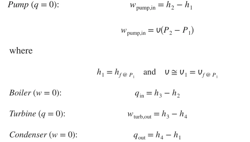
Solution steps:

1. To get different state variables, all the process parameters should be expressed such as all four processes occurring and the input parameter as state 1.
2. From the standard Xstem library to get the steam table data for water, most of the points in-between state variables are calculated and their corresponding parameters such as enthalpy, entropy, specific heat saturation temperature etc.
3. all the state points are used to find out the net work done, work done by the turbine, thermal efficiency back work ratio, etc according to their thermodynamic relations and necessary formulas.
4. To plot the property diagram of water, i.e saturation liquid and vapour line, an array is created using linspace command from 0 to value of t1 with 5000 evenly spaced points in between them and suitable state variables are iterated using for loop.
5. To plot T-s and H-s diagram all the required points are plotted and markd using text command.

Input parameters:

Turbine Inlet temperature = 400`degree` C

Turbine Inlet pressure = 30 bar

Turbine outlet pressure = 0.05bars = Condenser inlet pressure.

Main Program:

%A program for simulating Rankine cycle and plot required graphs.
close all
clear all
clc

%Subscript for different state points
% 1= Turbine inlet or boiler outlet, 2= Condenser inlet or turbine outlet,
%3 = Pump inlet or condenser outlet, 4= Boiler inlet or pump outlet

%Input paremeters:
%p1 = Turmine inlet pressur (bar)
%T1 = Temperature at turbine inlet(degree C)
%p2 = turbine outlet pressure(bar)


%description about process,
fprintf('Process (1-2) - Isentropic expension in the turbine')
fprintf('Process (2-3) - Isobaric heat rejection by the condenser')
fprintf('Process (3-4) - Isentropic compression in the pump')
fprintf('Process (4-1) - Isobaric heat addition by the boiler')

% For inputing state variable at point 1,
p1 = input('Enter the pressure at the turbine inlet (in bar):');
t1 = input('Enter the temperature at the turbine inlet (in degree celsius):');
p2 = input('Enter the pressure at the turbine outlet (in bar):');

% State variable at state poit 1(i.e turbine inlet)
h1 = XSteam('h_pT',p1,t1);  %Enthalpy in[KJ/Kg]
s1 = XSteam('s_pT',p1,t1);  %Specific entropy in[KJ/Kg K]
v1 = XSteam('v_pT',p1,t1);  %specific volume in[m3/Kg]

% State variable at state point 2(i.e Condenser inlet)
s2 = s1;  % specific entropy in[KJ/Kg K]
h2 = XSteam('h_px',p2,XSteam('x_ps',p2,s2));  %enthalpy in [KJ/Kg]
t2 = XSteam('T_ps',p2,s2);  %temperature in [degree C]
v2 = XSteam('v_ps',p2,s2);  %specific volume in [m3/Kg]

%state variable at state point 3(i.e pump inlet)
p3 = p2;  %pressure in[bar]
t3 = XSteam('Tsat_p',p3);  %temperature in [degreeV]
h3 = XSteam('hL_p',p3);  %enthalpy in [KJ/Kg]
s3 = XSteam ('sL_p',p3);  %specific entropy in[KJ/Kg K]
v3 = XSteam('vL_p',p3);  %inlet specific volume in [m3/Kg]

% State variable at state point 4 (i.e boiler inlet)
s4 = s3;  %specific entropy in[KJ/Kg K]
p4 = p1;  %pressure in[bar]
h4 = XSteam('h_ps',p4,s4);  %enthalpy in[KJ/Kg]
t4 = XSteam('T_ps',p4,s4);  %temperature in [degree C]
v4 = XSteam('v_ps',p4,s4);  %specific volume in [m3/Kg]


%After defining all the states noe lets process ech of these state and in
%between data variables
%Ploting graph for Ideal Rankine cycle 'T' vs's'.
figure(1)
hold on
plot([s1 s2],[t1 t2],'color','r','linewidth',5);
plot([s2 s3],[t2 t3],'color','k','linewidth',5);
plot([s1 s2],[t1 t2],'color','c','linewidth',5);
Trange = linspace(t4,t1,500);
for i = 1:length(Trange)
    s_range(i) = XSteam('s_pT',p1,Trange(i));
    h_range23(i) = XSteam('h_ps',p1,s_range(i));
    h_range41(i) = XSteam('h_ps',p2,s_range(i));
end
plot(s_range,Trange,'color','b','linewidth',5);
legend('Reversibleadiabaticexpansion','constantpressureheatrejection','reversibleisentropiccompression','constantpressure');


%ploting graph for ideal rankine cycle in 'h' vs 's'.
figure(2)
hold on
plot([s1 s2],[h1 h2],'color','r','linewidth',5);
plot(s_range,h_range23,'color','k','linewidth',5);
plot([s3 s4],[h3 h4],'color','c','linewidth',5);
plot(s_range,h_range41,'color','b','linewidth',5);
legend('Reversibleadiabaticexpansion','constantpressureheatrejection','reversibleisentropiccompression','constantpressure');


%ploting graphs for 'T' vs 's'
t_range = linspace(0,374.15,500);  %Temperature from 0 to critical point of water 
figure(1)
hold on
for i = 1:length(t_range)
    plot(XSteam('sL_t',t_range(i)),t_range(i),'.','color','g');
    plot(XSteam('sV_t',t_range(i)),t_range(i),'.','Color','g');
end

%ploting graph for 'h' vs's'
figure(2)
hold on
for i = 1:length(t_range)
    plot(XSteam('sL_t',t_range(i)),XSteam('hL_t',t_range(i)),'.','color','g');
    plot(XSteam('sV_t',t_range(i)),XSteam('hV_t',t_range(i)),'.','Color','g');
end

%ploting diagram for all state points for ideal rankine cycle in 'T' vs 's'

figure(1)
hold on
plot(s1,t1,'ko')
plot(s2,t2,'ko')
plot(s3,t3,'ko')
plot(s4,t4,'ko')
grid on
title('T-s diagram of rankine cycle')
xlabel('Temperature in [degree C]')


%Ploting diagram for all state points for ideal rankine cycle.
figure(2)
hold on
plot(s1,h1,'ko')
plot(s2,h2,'ko')
plot(s3,h3,'ko')
plot(s4,h4,'ko')
grid on
title('h-s diagram of rankine cycle')
xlabel('enthalpy in [KJ/Kg]')
ylabel('specific entropy in[KJ/Kg K]')

%finally calculating work efficiency
Work_turbine = h1 - h2;   %work transferred from the working fluid(KJ/Kg)
Q_taken_out_condenser = h2 - h3;  %Heat rejected from the working fluid (kj/kg)
Work_pump = h4 - h3;  %work transferred into the working fluid(kl/kg)
Q_given_boiler = h1 - h4;  %heat transferred to the working fluid(kj/kh)
Back_Work_Ratio = Work_turbine / Work_pump;  %back work ratio
SSE = 3600/(Work_turbine - Work_pump);  %speciic steam consumption (kg/kwg)
Work_net = Work_turbine - Work_pump;  %net work on the working fluid (kj/kg)
Effi_rankine = Work_net/Q_given_boiler;  %rankine cycle efficiency

clc
% printing result to the user giving input
fprintf('**********************RANKINE CYCLE:IDEAL CYCLE FOR VAPOUR POWER CYCLE********');

fprintf('PROCESS 1-2:REVERSIBLE ADIABTIV ECPENCION PROCESS IN THE STEAM TURBINE');
fprintf('Process 2-3: constant pressure heat transfer process in the condensern');
fprintf('process3-4:reversible adiabatic compression process in the pump');
fprintf('process4-1:constant pressure heat transfer process in the boiler');

fprintf('-------------state variable at state point 1-------------');
fprintf('turbine inlet temperature T1 = %.5f in degree c',t1);
fprintf('Turbine inlet presure p1 = %.5f in bar',p1);
fprintf ('Turbine inlet enthalpy h1 = %.5f in kj/kg',h1);
fprintf('Turbine inlet specific entropy s1 = %.5f in kj/kg k',s1);
fprintf('Turbine inlet specific volume v1 = %.5f in m3/kg',v1);

fprintf('-------------state variable at state point 2-------------');
fprintf('Condenser inlet temperature T2 = %.3f in degree c',t2);
fprintf('Condenser inlet presure p2 = %.3f in bar',p2);
fprintf ('Condenser inlet enthalpy h2 = %.3f in kj/kg',h2);
fprintf('Condenser inlet specific entropy s2 = %.3f in kj/kg k',s2);
fprintf('Condenser inlet specific volume v2 = %.3f in m3/kg',v2);

fprintf('-------------state variable at state point 3-------------');
fprintf('Pump inlet temperature T3 = %.3f in degree c',t3);
fprintf('Pump inlet presure p3 = %.3f in bar',p3);
fprintf ('Pump inlet enthalpy h3 = %.3f in kj/kg',h3);
fprintf('Pump inlet specific entropy s3 = %.3f in kj/kg k',s3);
fprintf('Pump inlet specific volume v3 = %.3f in m3/kg',v3);

fprintf('-------------state variable at state point 4-------------');
fprintf('Boiler inlet temperature T4 = %.3f in degree c',t4);
fprintf('Boiler inlet presure p4 = %.3f in bar',p4);
fprintf ('Boiler inlet enthalpy h4 = %.3f in kj/kg',h4);
fprintf('Boiler inlet specific entropy s4 = %.3f in kj/kg k',s4);
fprintf('Boiler inlet specific volume v4 = %.3f in m3/kg',v4);

fprintf('-----------Work and Efficiency--------');
fprint('Work transferred from the working fluid wturbine = %.4f in kj/kg',Work_turbine);
fprint('heat rejected from the working fluid Qcondenser = %.4f in kj/kg',Q_taken_out_condenser);
fprintf('work transferred into the working fluid wpump = %.4f in kj/kg',Work_pump);
fprintf('heat transferred to the working fluid Qboiler = %.4f in kj/kg',Q_given_boiler);

fprintf('Back work ratio BWR = %.4f',Back_Work_Ratio);
fprintf('specific steam consumption SSE = %.4f in kj/kg',SSE);
fprintf('net work on the working fluid Wnet = %.4f in kj/kg',work_net);
fprintf('rankine cycle efficiency ETArankine = %.4f',Effi_rankine*100);

fprintf('-----------------------SUCCESSFULLY DONE THE CALCULATIONS-----------');

RESULT: