Project 2 - Rankine cycle Simulator

%% Rankine Cycle Simulation using Matlab

% Taking the Thermal properties using Xsteam data file
% To calculate the work done by turbine, pump, net workdone, efficiency
clear all
close all
clc

%% Rankine Cycle Process

%Process 1-2 is Isentropic Expansion ( Turbine )
% Process 2-3 is Constant Pressure heat reduction ( Condensor )
%Process 3-4 is Isentropic Compression ( Pump )
% Process 4-1 is Constant pressure Heat addition ( boiler )

% displaying the process of Rankine cycle
disp( 'Rankine Cycle Process' )
disp('Process 1-2 is Isentropic Compression in Turbine' )
disp('process 2-3 is Constant pressure Heat reduction in the Condensor' )
disp( 'process 3-4 is Isentropic Expansion in Pump')
disp( 'Process 4-1 is Constant Pressure heat addition in Boiler' )


%% Inputs

% Inputs pressure is taken in 'bar', Temperature is taken in 'degree Celcius'
% values of pressure and temperature.

T3 = input( 'Inlet Temperature for Turbine T3(C) = ')
p3 = input('Inlet Pressure of the Turbine p3(bar) = ')
p4 = input('Outlet Pressure of the Turbine p4(bar) = ')

%% State_Points

% by using XSteam library we are taking the required data like pressure, temperature, entropy, enthalpy

% State 1 Inputs

T1 = XSteam( 'Tsat_p' , p4);
p1 = p4;
h1 = XSteam( 'hL_p' , p4);
s1 = XSteam( 'sL_p' , p4);


% State_2 Inputs


T2 = XSteam( 'Tsat_p' , p3, s1);
p2 = p3;
h2 = XSteam( 'h_ps' , p3, s1);
s2 = s1;


% State 3 Inputs

h3 = XSteam( 'h_pT' , p3, T3);
s3 = XSteam( 's_pT' , p3, T3);


% State_4 Inputs
sg4 = XSteam('sV_p', p4)-XSteam('sL_p', p4);
hg4 = XSteam('hV_p', p4)-XSteam('hL_p', p4);
s4 = s3;
X = (s4-s1)/sg4;
h4 = h1+(X*hg4);
v4 = XSteam( 'VL_p', p4);
T4 = XSteam( 'T_ph' , p4, h4);


%Intermediate State points

T5 = XSteam( 'Tsat_p', p3);
h5 = XSteam( 'hL_p' , p3);
s5 = XSteam( 'sL_p' , p3);
T6 = XSteam( 'Tsat_p' , p3);
h6 = XSteam( 'hv_p', p3);
s6 = XSteam( 'sV_p' , p3);
P5 = p3;
p6 = p3;

%% calculating work done

% workdone by Turbine
W_t = h3-h4;

% workdone by Pump
W_p = v4*(p3 -p4)*100;
hf2 = W_p + h1;

% Calculating Net workdone
W_net = W_t-W_p;

%% Calculating Heat in to the system
Q_in = h3-h2;

%% Calculating Thermal Efficiency 
n_eff = (W_net/Q_in)*100;

%% Calculating specific steam consumption (SSC) = mass flow rate/net workdone
SSC = (3600/W_net);

%% Calculating Back Work Ratio
B_w = (W_p/W_t);


%% Plot for the Saturation Curve

S = linspace(0.1,10, 1000);
for i = 1: length(S)
Tsat (i) = XSteam('Tsat_s' ,S(i));
end

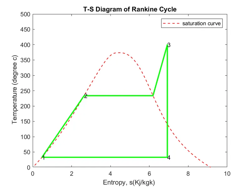
%% Plotting T-S diagram

figure(1)
plot (S, Tsat, ' -- ', 'Linewidth', 1, 'color', 'r')
hold on
plot ( [ s1, s5, s5, s6, s3, s4, s1], [T1, T2, T5, T6, T3, T4, T1], 'linewidth' , 2, 'color' , 'g')
xlim([0 10])
ylim([0 500])
title('T-S Diagram of Rankine Cycle')
xlabel( 'Entropy, s(Kj/kgk) ' )
ylabel ( ' Temperature (degree c)')
legend( 'saturation curve' )
hold off

% marking State points
text (s1, T1, "1");
text (s5, T2, "2");
text (s3, T3, "3");
text (s4, T4, "4") ;


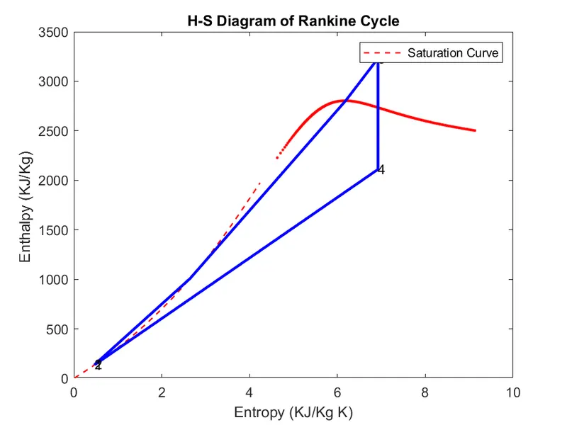
%% Plotting H_S diagram
T = (1:2000);
for j = 1: length(T)
h_L(1,j) = XSteam('hL_T' , j);
h_V(1, j) = XSteam('hV_T' , j);
s_L(1, j) = XSteam('sL_T', j);
s_V(1,j) = XSteam('sV_T', j);
end

figure(2)
plot (s_L, h_L, '--', 'Linewidth',1, 'color' , 'r')
hold on
plot (s_V, h_V, '.', 'Linewidth', 1, 'color', 'r')
plot ([s1, s2, s5,s6, s3, s4, s1],[h1, h2, h5, h6, h3, h4, h1], 'linewidth', 2, 'color', 'b')
title('H-S Diagram of Rankine Cycle' )
xlabel('Entropy (KJ/Kg K)' )
ylabel('Enthalpy (KJ/Kg) ' )
legend( 'Saturation Curve' )

%marking state points
text (s1, h1, "1");
text (s2, h2, "2")
text (s3, h3, "3" ) ;
text (s4, h4, "4" )

saveas (1, 'T-S Diagram of Rankine Cycle', 'png' )
saveas (2, 'H-S Diagram of Rankine Cycle' , 'png')

%% Results
disp('Results' );
p3 = p3;
p4 = p4;
T3 = T3;

% Stage point 1
disp('At stage point 1');
S_p1 = sprintf('p1 is %.3f bar', p1);
disp(S_p1);
S_T1 = sprintf('T1 is %.3f "c', T1);

disp(S_T1);
S_h1 = sprintf('h1 is %.3f <3/kg', h1);
disp (S_h1) ;
S_s1 = sprintf('s1 is %.3f KJ/kg K', s1);
disp(S_s1) ;

% Stage point 2
disp('At stage point 2') ;
S_p2 = sprintf('p2 is %. 3f bar' , p2);
disp(S_p2);
S_T2 = sprintf('T2 is X.3f C', T2);
disp(S_T2);
S_h2 = sprintf('h2 is %.3f KJ/Kg', h2);
disp(S_h2) ;
S_s2 = sprintf('s2 is X.3f K3/Kg K', s2);
disp(S_s2);


% Stage point3

disp('At stage point 3');
S_p3 = sprintf('p3 is %.3f bar', p3);
disp(S_p3) ;
S_T3 = sprintf('13 is %.3f C', T3);
disp(S_T3) ;
S_h3 = sprintf('h3 is %.3f KJ/kg', h3);
S_T3 = sprintf('T3 is %.3f C', 13);
disp(S_T3);
S_h3 = sprintf('h3 is %. 3f <3/kg', h3);
disp(S_h3);
S_s3 = sprintf('s3 is %.3f KJ/kg K', s3);
disp(S_s3);


% Stage point 4
disp('At stage point 4');
S_p4 = sprintf('p4 is %.3f bar', p4);
disp(S_p4);
S_T4 = sprintf('T4 is %.3f C', 14);
disp(S_T4);
S_h4 = sprintf('h4 is %.3f KJ/kg', h4);
disp(S_h4);
S_s4 = sprintf('s4 is %.3f KJ/kg K', 54);
disp(S_s4);

%%  Efficiency and Back work ratio

wt = sprintf('wt is %.3f KJ/Kg', W_t);
disp(wt) ;
Wp = sprintf('wp is %.3f KJ/Kg', W_p);
disp(Wp) ;
w_net = sprintf('W_net is %. 3f KJ/Kg', W_net);
disp (W_net);
neff = sprintf('Thermal Efficiency is %.3f percent', n_eff);
disp(neff);
Ssc = sprintf('SSC is %.2f kg/KWh', SSC);
disp(Ssc);
BW = sprintf('Back Work Ratio is %.3f', B_w);
disp(BW) ;

Explanation of Code:

Firstly, we displayed the process of Rankine cycle by using disp command.

By using the command input we are giving the values of pressure and temperature, inputs (p3, T3, p4) which are pressure values at inlet & outlet of turbine, Inlet Temperature of the turbine.

Then used the XSteam library we are taking the required data like pressure, temperature, enthalpy and entropy .

Loaded all the data then calculated the net work done, thermal efficiency, Specific Steam Consumption and back work ratio.

by using plot command , ploted the saturation curve for the saturation curve we are using for loop to determine the curve , T-S and H-S diagrams.

Used xlim' and ylim' commands we are specifying the limits of xaxis and yaxis

Labelled the plot by used title, xlabel, ylabeland legend commands.

For creating the state points, we used a command called 'text, which indicates the state points.

saved the plot by used saveas

errrors faced :

common errors faced are spelling mistakes

setting the limit ( didnt get the proper graph because of improper limits )