Project 2 - Rankine cycle Simulator
REPORT:
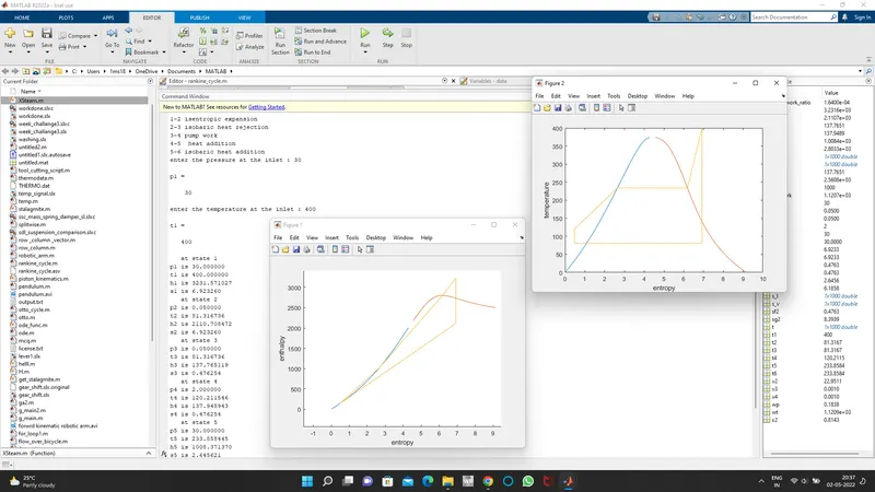
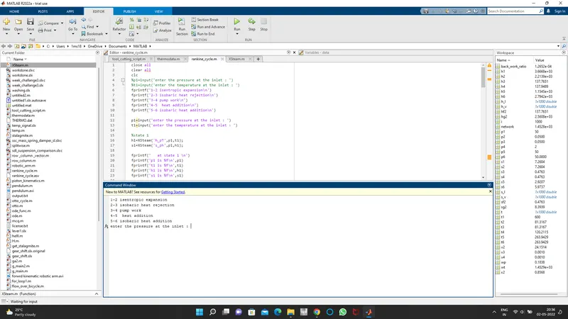
- inputs(state points at the inlet of the turbine) are taken by the user using input.
p1=input('enter the pressure at the inlet : ')t1=input('enter the temperature at the inlet : ')
- state points at different states are calculated by using XSteam.
h1=XSteam('h_pT',p1,t1);s1=XSteam('s_ph',p1,h1);
3. entropy and enthalpy values for different temperature values are calculated by using for loop for both vapor and liquid states.
t=linspace(0,600,1000);
for i=1:length(t)
s_l(i)=XSteam('sL_T',t(i)); %at saturated liquid state
h_l(i)=XSteam('hL_T',t(i));
s_v(i)=XSteam('sV_T',t(i)); %at saturated vapour state
h_v(i)=XSteam('hV_T',t(i));
end
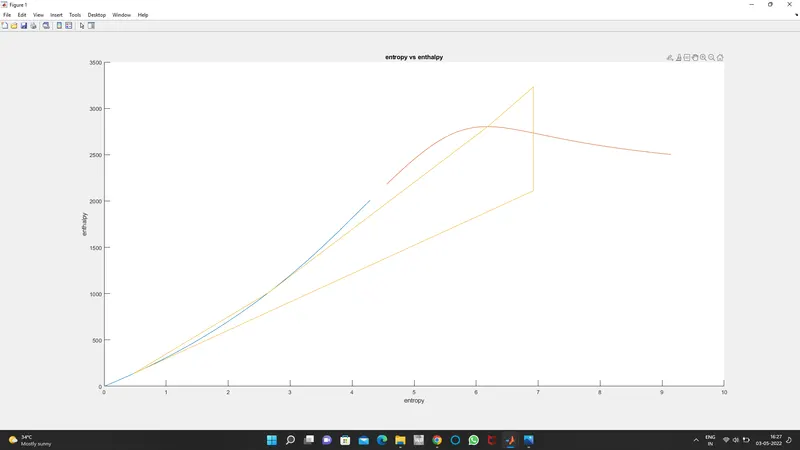
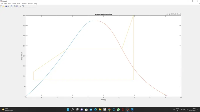
4.TS and HS graphs are plotted
%plotting
% HS plot
hold on
figure(1)
plot(s_l,h_l)
plot(s_v,h_v)
plot([s1 s2 s3 s4 s5 s6 s1],[h1 h2 h3 h4 h5 h6 h1])
xlabel('entropy')
ylabel('enthalpy')
hold off
% TS plot
figure(2)
plot(s_l,t)
hold on
plot(s_v,t)
plot([s1 s2 s3 s4 s5 s6 s1],[t1 t2 t3 t4 t5 t6 t1])
xlabel('entropy')
ylabel('temperature')
Errors:
errors are due to syntax
these are corrected by changing the syntax.
Rankine Cycle:
it is the thermodynamic cycle that is used in heat engines(steam engines, reciprocating).
Rankine cycle is formed by four main components these are pump, boiler, turbine, and condenser.
pump is used to pump the working liquid to the boiler in which liquid is heated to saturate or superheated state which is then passed through a turbine to rotate in turn generates the electricity. the condenser is used to condense the superheated steam to the liquid state. then the liquid is passed to the pump. process repeats.
it is operated in four cycles that include two isentropic and two isobaric processes.
1-2 isentropic expansion
2-3 constant pressure heat rejection.
3-4 isentropic compression.
4-1 constant pressure heat addition.
Rankine cycle is modified to enhance the efficiency in following ways,
- reheat
- regeneration.
close all clear all clc fprintf('1-2 isentropic expansion\n') fprintf('2-3 isobaric heat rejection\n') fprintf('3-4 pump work\n') fprintf('4-5 heat addition\n') fprintf('5-6 isobaric heat addition\n') % input to the turbine p1=input('enter the pressure at the inlet : ') t1=input('enter the temperature at the inlet : ') %state 1 h1=XSteam('h_pT',p1,t1); s1=XSteam('s_ph',p1,h1); fprintf(' at state 1 \n') fprintf('p1 is %f\n',p1) fprintf('t1 is %f\n',t1) fprintf('h1 is %f\n',h1) fprintf('s1 is %f\n',s1) %state 2 p2=0.05; s2=s1; t2=XSteam('Tsat_p',0.5); sf2=XSteam('sL_p',p2); sg2=XSteam('sV_p',p2); hf2=XSteam('hL_p',p2); hg2=XSteam('hV_p',p2); x2=((s2-sf2)/(sg2-sf2)); h2=hf2+x2*(hg2-hf2); v2=XSteam('v_ph',p2,h2); fprintf(' at state 2 \n') fprintf('p2 is %f\n',p2) fprintf('t2 is %f\n',t2) fprintf('h2 is %f\n',h2) fprintf('s2 is %f\n',s2) %state 3 p3=p2; t3=t2; s3=XSteam('sL_p',p3); h3=XSteam('hL_p',p3); v3=XSteam('v_ph',p3,h3); fprintf(' at state 3 \n') fprintf('p3 is %f\n',p3) fprintf('t3 is %f\n',t3) fprintf('h3 is %f\n',h3) fprintf('s3 is %f\n',s3) %state 4 s4=s3; p4=2; v4=XSteam('v_ps',p4,s4); h4=XSteam('h_ps',p4,s4); t4=XSteam('Tsat_p',p4); fprintf(' at state 4 \n') fprintf('p4 is %f\n',p4) fprintf('t4 is %f\n',t4) fprintf('h4 is %f\n',h4) fprintf('s4 is %f\n',s4) %state 5 p5=p1; t5=XSteam('Tsat_p',p5); s5=XSteam('sL_p',p5); h5=XSteam('hL_T',t5); fprintf(' at state 5 \n') fprintf('p5 is %f\n',p5) fprintf('t5 is %f\n',t5) fprintf('h5 is %f\n',h5) fprintf('s5 is %f\n',s5) %state 6 t6=t5; p6=XSteam('psat_T',t6); s6=XSteam('sV_p',p6); h6=XSteam('hV_p',p6); fprintf(' at state 6 \n') fprintf('p6 is %f\n',p6) fprintf('t6 is %f\n',t6) fprintf('h6 is %f\n',h6) fprintf('s6 is %f\n',s6) wt=h1-h2; %turbine work wp=h4-h3; %pump work back_work_ratio=wp/wt; %back work ratio network=wt-wp; %network output fprintf('net work done is : %f',network ) fprintf('\n back work ratio is : %f',back_work_ratio) % property values at different temperature t=linspace(0,600,1000); for i=1:length(t) s_l(i)=XSteam('sL_T',t(i)); %at saturated liquid state h_l(i)=XSteam('hL_T',t(i)); s_v(i)=XSteam('sV_T',t(i)); %at saturated vapour state h_v(i)=XSteam('hV_T',t(i)); end %plotting % HS plot hold on figure(1) plot(s_l,h_l) plot(s_v,h_v) plot([s1 s2 s3 s4 s5 s6 s1],[h1 h2 h3 h4 h5 h6 h1]) xlabel('entropy') ylabel('enthalpy') title('entropy vs enthalpy') hold off % TS plot figure(2) plot(s_l,t) hold on plot(s_v,t) plot([s1 s2 s3 s4 s5 s6 s1],[t1 t2 t3 t4 t5 t6 t1]) xlabel('entropy') ylabel('temperature') title('entropy vs temperature')