Challenge

Project 2 - Rankine cycle Simulator

PPoojith Gowda29 Apr 2022

PRJECT : RANKINE CYCLE SIMULTOR

AIM : To Create a Rankine cycle simulator using matlab / Octave.

OBJECTIVE :

1.Code the basic program that calculates the state points alone

2.Then add the thermodynamic relation to get the points inbetween the state variables.

EXPLANATION ABOUT THE RANKINE CYCLE

The four processes of an ideal Rankine cycle are as follows;

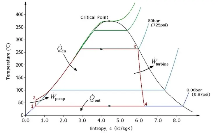
Process 1-2: Isentropic compression in a pump. Here the working fluid is pumped from low to high pressure.
2-3: Constant pressure heat addition in the boiler. In this process, the high-pressure liquid is added to the boiler and is heated at constant pressure to become a dry saturated vapour.
3-4: Isentropic expansion in a turbine. The dry saturated vapour expands through the turbine resulting in the generation of power.
4-1: Constant pressure heat rejection in a condenser. Wet vapour is condensed at a constant pressure to become a saturated liquid.

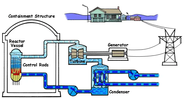
DETAILED DRAWING EXAMPLE FOR RANKINE CYCLE :

PV DIGRAM EXPLANATION FOR THE RANKINE CYCLE :

The efficiency of power cycles is defined as

Values of heat and work can be determined by applying the First Law of Thermodynamics to each step. The steam quality x at the turbine outlet is determined from the assumption of isentropic expansion, i.e.,

where is the entropy of vapor and Si* the entropy of liquid.

Inefficiencies of Real Rankine Cycles

The efficiency of the ideal Rankine cycle as described in the previous section is close to the Carnot efficiency (see Carnot Cycle). In real plants, each stage of the Rankine cycle is associated with irreversible processes, reducing the overall efficiency. Turbine and pump irreversibilities can be included in the calculation of the overall cycle efficiency by defining a turbine efficiency according to Figure 3

where subscript act indicates actual values and subscript is indicates isentropic values and a pump efficiency

Turbine efficiency.

If η_t and η_p are known, the actual enthalpy after the compression and expansion steps can be determined from the values for the isentropic processes. The turbine efficiency directly reduces the work produced in the turbine and, therefore the overall efficiency. The inefficiency of the pump increases the enthalpy of the liquid leaving the pump and, therefore, reduces the amount of energy required to evaporate the liquid. However, the energy to drive the pump is usually more expensive than the energy to feed the boiler.

Rankine cycle with vapor superheating.

Even the most sophisticated boilers transform only 40% of the fuel energy into useable steam energy. There are two main reasons for this wastage:

The combustion gas temperatures are between 1000°C and 2000°C, which is considerably higher than the highest vapor temperatures. The transfer of heat across a large temperature difference increases the entropy.
Combustion (oxidation) at technically feasible temperatures is highly irreversible.

Since the heat transfer surface in the condenser has a finite value, the condensation will occur at a temperature higher than the temperature of the cooling medium. Again, heat transfer occurs across a temperature difference, causing the generation of entropy. The deposition of dirt in condensers during operation with cooling water reduces the efficiency.

Increasing the Efficiency of Rankine Cycles

Pressure difference

The net work produced in the Rankine cycle is represented by the area of the cycle process in Figure . Obviously, this area can be increased by increasing the pressure in the boiler and reducing the pressure in the condenser.

Superheating and reheating

The irreversibility of any process is reduced if it is performed as close as possible to the temperatures of the high temperature and low temperature reservoirs. This is achieved by operating the condenser at subatmospheric pressure. The temperature in the boiler is limited by the saturation pressure. Further increase in temperature is possible by superheating the saturated vapor, see Figure

This has the additional advantage that the vapor quality after the turbine is increased and, therefore the erosion of the turbine blades is reduced. It is quite common to reheat the vapor after expansion in the high pressure turbine and expand the reheated vapor in a second, low pressure turbine.

Feed water preheating

The cold liquid leaving the feed pump is mixed with the saturated liquid in the boiler and/or re-heated to the boiling temperature. The resulting irreversibility reduces the efficiency of the boiler. According to the Carnot process, the highest efficiency is reached if heat transfer occurs isothermally. To preheat the feed liquid to its saturation temperature, bleed vapor from various positions of the turbine is passed through external heat exchangers (regenerators), as shown in Figure .

Ideally, the temperature of the bleed steam should be as close as possible to the temperature of the feed liquid.

Combined cycles

The high combustion temperature of the fuel is better utilized if a gas turbine or Brayton engine is used as "topping cycle" in conjunction with a Rankine cycle. In this case, the hot gas leaving the turbine is used to provide the energy input to the boiler. In co-generation systems, the energy rejected by the Rankine cycle is used for space heating, process steam or other low temperature applications.

..............................................

PROGRAM AND EXPLANATION.

% steam table data has been provided with Xteam file

% Prgram for Simulating rankine cycle as fallows

clear all
close all
clc

% Output Header

disp(' RANKIN CYCLE SIMULATOR')
disp('1-2 Isentropic Expansion in the Turbine')
disp('2-3 Constant Pressure Heat rejection process')
disp('3-4 Isentropic compression process in the Pump')
disp('4-1 Constant Pressure Heat addition process')

% Taking the input from the User

p1=input('Enter the Pressure at the Turbine Inlet(in Bar): ');
T1=input('Enter the Temperature at the Turbine Inlet (in Celcius): ');
p2=input('Enter the Pressure at the Condenser Inlet (in Bar): ');
sf1=XSteam('sL_p',p1);
sg1=XSteam('sV_p',p1);
sf2=XSteam('sL_p',p2);
sg2=XSteam('sV_p',p2);
hf2=XSteam('sL_p',p2);
hg2=XSteam('sV_p',p2);

Temp_03=XSteam('T_ps',p1',sf1);

if T1<=Temp_03
disp('the cycle can not have if %f as inlet temperature',T1);
disp(f)

else
%state point 1

s1=XSteam('s_pT',p1,T1);
h1=XSteam('h_pT',p1,T1);
s2=s1;
x2=(s2-sf2)/(sg2-sf2);
h2=hf2+(x2*(hg2-hf2));
p3=p2;
h3=XSteam('hL_p',p3);
s3=XSteam('sL_p',p3);
T3=XSteam('Tsat_p',p3);
T2=T3;
v3=XSteam('vL_p',p3);

%state point 4
%inlet pressure of the turbine=outlet pressure of the pump
p4=p1;
s4=s3; %entropy at the pump inlet=entropy at the pump outlet
T4=XSteam('T_ps',p4,s4); %outlet temperature of the pump

% Pump work

Wp=v3*(p4-p3)*100; %amount of work required for the pump

h4=h3+Wp %enthalpy at the inlet of the boiler

%work output

Wt=h1-h2; %Work done by the turbine
Wnet=Wt-Wp; %net work

%Heat input

Qin=h1-h4;
%Heat rejected in the condenser

Qout=h2-h3;

% Thermal efficiency

ntherm=Wnet/Qin;

%calculation for the T-S curve for the water
Pressure=linspace(0,1000,6000) %Pressure range for the culculating the T-S curve for the water
for i=1:length(Pressure)
EntropyL(i)=XSteam('sL_P',Pressure(i));
Temperature(i)=XSteam('Tsat_P',Pressure(i));
EntropyV(i)=XSteam('sV_P',Pressure(i));
end

%Calulating the T-S curve for the inlet pressure

e_1_p1=linspace(sf2,sf1,100);
e_2_p1=linspace(sg1,s1,100);
for i=1:length(e_1_p1)
Temp_01(i)=XSteam('T_ps',p1,e_1_p1(i));
Temp_02(i)=XSteam('T_ps',p1,e_2_p1(i));
end

%Calculating state points and T- s curve for the Water

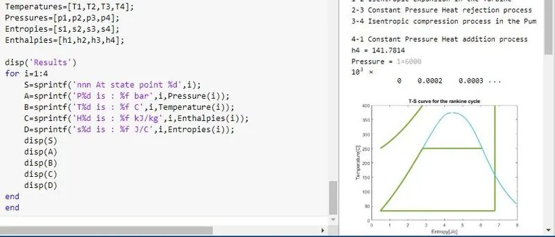
figure(1)
plot([s1 s2],[T1 T2],'color','#77AC30','linewidth',3);
hold on
title('T-S curve for the rankine cycle')
xlabel('Entropy[J/c]');
ylabel('Temperature[C]');
plot([s2 s3],[T2 T3],'color','#77AC30','linewidth',3);
plot([s3 s3],[T3 T4],'color','#77AC30','linewidth',3);
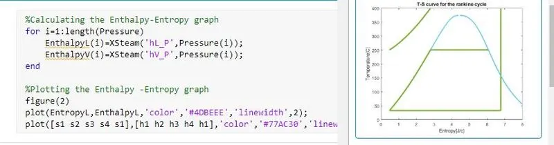
plot(EntropyL,Temperature,'color','#4DBEEE','linewidth',2);
plot(EntropyV,Temperature,'color','#4DBEEE','linewidth',2);
plot(e_1_p1,Temp_01,'color','#77AC30','linewidth',3);
plot(e_1_p1,Temp_02,'color','#77AC30','linewidth',3);
plot([sf1 sg1],[Temp_03 Temp_03],'color','#77AC30','linewidth',3);

%Calculating the Enthalpy-Entropy graph
for i=1:length(Pressure)
EnthalpyL(i)=XSteam('hL_P',Pressure(i));
EnthalpyV(i)=XSteam('hV_P',Pressure(i));
end

%Plotting the Enthalpy -Entropy graph
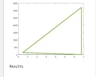
figure(2)
plot(EntropyL,EnthalpyL,'color','#4DBEEE','linewidth',2);
plot([s1 s2 s3 s4 s1],[h1 h2 h3 h4 h1],'color','#77AC30','linewidth',3);

%Print the out put

Temperatures=[T1,T2,T3,T4];
Pressures=[p1,p2,p3,p4];
Entropies=[s1,s2,s3,s4];
Enthalpies=[h1,h2,h3,h4];

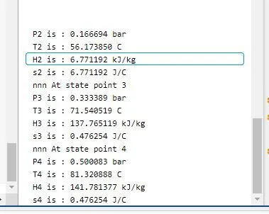
disp('Results')
for i=1:4
S=sprintf('nnn At state point %d',i);
A=sprintf('P%d is : %f bar',i,Pressure(i));
B=sprintf('T%d is : %f C',i,Temperature(i));
C=sprintf('H%d is : %f kJ/kg',i,Enthalpies(i));
D=sprintf('s%d is : %f J/C',i,Entropies(i));
disp(S)
disp(A)
disp(B)
disp(C)
disp(D)
end
end

OUT PUT :