Project 2 - Rankine cycle Simulator
AIM
To simulate Rankine cycle with Turbine input and output condition using Matlab and steam Data function file
Introduction
The Rankine cycle is the fundamental operating cycle of all power plants where an operating fluid is continuously evaporated and condensed. The selection of operating fluid depends mainly on the available temperature range.
The Rankine cycle system consists of a pump, boiler, turbine, and condenser. The pump delivers liquid water to the boiler. The boiler heated by the solar heat converts water to superheated steam. This steam is used to run the turbine which powers the generator. Steam leaves the turbine and becomes cooled to a liquid state in the condenser. Then the liquid is pressurized by the pump and goes back to the boiler. And the cycle continues.
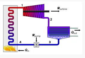
In an ideal Rankine cycle, all the units operate with the steady-state flow, and the kinetic and potential energy of the fluid is considered to be negligible compared to the temperature and pressure effects.
Process
1-2 Isoentropy Expansion in turbine
2-3 Isobaric heat rejection by condensor
3-4 Isoentropy compression in pump
4-1 Isobaric heat Supply by the boiler
Enthalpy H
enthalpy H is defined as the sum of its internal energy and the product of its pressure and volume
`H=U+PV`
Entropy S
Entropy is a measurable physical property that is most commonly associated with a state of disorder, randomness, or uncertainty.
1-2 Isoentropy Expansion in turbine
expansion of the steam in the turbine. The work done through that process is the useful work, which is the main purpose of the cycle
Work done is
`W_T=H1-H2`
Here, we again assume that there is no heat exchange with the surrounding, so all the fluid energy change is converted to work. Note that the enthalpy change is written as "before" minus "after" because the energy of the superheated compressed steam is higher than the expanded steam after it exits the turbine. So, this expression gives us a positive work value.
where the stream is a Dry stream
2-3 Isobaric heat rejection by condensor
steam cooling and condensation. The energy balance on the condenser will be
`Q_R=H4-H1 (KJ)/(kg)`
constant pressure heat rejection
where there is no work done only energy transfer and phase change obtain
3-4 Isoentropy compression in pump
we assume there is no heat exchange with the surroundings, so the energy is not lost (which is an ideal scenario). The process, which is not accompanied by any heat exchange with the environment, is termed "adiabatic." So, this step is an adiabatic compression.
`W_p=H4-H3 (KJ)/(kg)`
the volume of the stream is calculated by in pressure of the pump from the steam function value
4-1 Isobaric heat Supply by the boiler
takes place in the boiler. The energy balance in the boiler can be expressed as the change in enthalpy of the fluid from the "before" state (compressed liquid) to the "after" state (superheated steam) which is 5 (dry stream) & 6 (superheat stream)
Heat is added at constant pressure
`QS=H1-H4 (KJ)/(kg)`
WORK DONE
`W_(NET)=WORKDONE BY TURBINE (W_T) + WORK DONE BY PUMP (W_P) (KJ)/kg`
Efficiency of system
`\eta=(WORK DONE)/(HEAT SUPPLY)*100 %`
STREAM RATE FOR TURBINE
`SST=3600/(W_T-W_P) (KJ)/(kwh)`
Back Pressure Ratio
Back work ratio = Pump work/Turbine work
MATLAB
COAD
clear all;
close all;
clc;

% process
fprintf('                               Rankine cycle Simulator')
fprintf('\nProcess\n');
fprintf('1-2 Isoentropy Expansion in turbine\n');
fprintf('2-3 Isobaric heat rejection by condensor\n');
fprintf('3-4 Isoentropy compression in pump \n');
fprintf('4-1 Isobaric heat Supply by boiler\n');


% Input condition
fprintf('\n Input condition \n')
P1=input('Enter the Pressure at turbine inlet {in bar] P1:');
T1=input('Enter the Temperature at turbine inlet {in degree celcius] T1:');
P2=input('Enter the Pressure at condensor inlet {in bar] P2:');

% step2 calculate value from function file
%state point1
H1=XSteam('h_pt',P1,T1);
S1=XSteam('s_pt',P1,T1);

%step3 state point2
S2=S1;
sf2=XSteam('sL_p',P2);
sg2=XSteam('sV_p',P2);
hf2=XSteam('hL_p',P2);
hg2=XSteam('hV_p',P2);
S2=sg2;
H2=hg2;
T2=XSteam('T_hs',H2,S2);

% turbine workdone
wt=H1-H2;

%step4 state point 3
T3=T2;
P3=P2;
S3=XSteam('sL_T',T3);
H3=XSteam('hL_T',T3);
V3=XSteam('vL_P',P3);
% work done by pump
wp=V3*(P1-P2)*100;
% net work done
w_net=wt-wp;
% steam rate
steam_rate=3600/(wt-wp);

%step 5 state point 4
P4=P1;
S4=S3;
cp4=XSteam('Cp_ps',P4,S4);
cv4=XSteam('Cv_ps',P4,S4);
% from Ideal gas adiabatic process
gamma=cp4/cv4;
r= (gamma-1)/gamma;
T4=T3*(P4/P3)^r;
H4=wp+H3;
% heat supply
Qs=H1-H4;
% efficiency
eta=w_net/Qs*100;

% Back work ratio
BWR= wp/wt;
% step 7 state point 5 & 6
T5=XSteam('Tsat_p',P1);
T6=T5;
S5=XSteam('sL_p',P1);
S6=XSteam('sV_p',P1);
H5=XSteam('hL_p',P1);
H6=XSteam('hV_p',P1);

% print result at all points
fprintf('\n---------------------Result---------------\n');
fprintf('At  State point 1;\nP1 = %4.2f bar;\nT1 = %4.2f degree celcius;\nh1 = %4.2f kj/kg;\ns1 = %4.2f kj/kgk;\n\n',P1,T1,H1,S1)
fprintf('At  State point 2;\nP2 = %4.2f bar;\nT2 = %4.2f degree celcius;\nh2 = %4.2f kj/kg;\ns2 = %4.2f kj/kgk;\n\n',P2,T2,H2,S2)
fprintf('At  State point 3;\nP3 = %4.2f bar;\nT3 = %4.2f degree celcius;\nh3 = %4.2f kj/kg;\ns3 = %4.2f kj/kgk;\n\n',P3,T3,H3,S3)
fprintf('At  State point 4;\nP4 = %4.2f bar;\nT4 = %4.2f degree celcius;\nh4 = %4.2f kj/kg;\ns4 = %4.2f kj/kgk;\n\n',P4,T4,H4,S4)
fprintf('wt = %4.2f kj/kg;\n wp = %4.2f kj/kg;\n wnet =%4.2f kj/kg;\n eta_thermal=%4.2f%%;\n SSC=%4.2f kj/kwh;\n BWR=%4.4f;',wt,wp,w_net,eta,steam_rate,BWR)

% line point creation in between Temperature (T5 to T1)
T_line=linspace(T5,T1,500);
% line point creation in between entropy (H5 to H1)
for i=1:length(T_line)
    S_line(i)=XSteam('s_pT',P1,T_line(i));
end
% curve creation for saturated property
T_SAT=linspace(1,500,500);
for j=1:length(T_SAT)
    Sl(j)=XSteam('sL_t',T_SAT(j));
    Sv(j)=XSteam('sV_t',T_SAT(j));
    Hl(j)=XSteam('hL_t',T_SAT(j));
    Hv(j)=XSteam('hV_t',T_SAT(j));
end
subplot(1,2,1)
plot([S1 S2 S3 S4 S5 S6 S_line],[T1 T2 T3 T4 T5 T6 T_line],'linewidth',2);
hold on;
plot(Sl,T_SAT,'r');
plot(Sv,T_SAT,'r');
ylim([0 450])
xlabel('Entropy S (kj/kg)')
ylabel('Temperature T (degree c)')
text(S1,T1,'1','FontSize',13)
text(S2,T2,'2','FontSize',13)
text(S3,T3,'3','FontSize',13)
text(S4,T4,'4','FontSize',13)
text(S5,T5,'5','FontSize',13)
text(S6,T6,'6','FontSize',13)
title('S Vs T ')
subplot(1,2,2)
plot([S1 S2 S3 S4 S1],[H1 H2 H3 H4 H1],'linewidth',2);
hold on
plot(Sl,Hl);
plot(Sv,Hv);
xlabel('Entropy H (kj/kg)')
ylabel('Enthalphy S (kj/kgk)')
text(S1,H1,'1','FontSize',13)
text(S2,H2,'2','FontSize',13)
text(S3,H3,'3','FontSize',13)
text(S4,H4,'4','FontSize',13)
text(S5,H5,'5','FontSize',13)
text(S6,H6,'6','FontSize',13)
title('S Vs H')
Command Used
- fprintf - display strings or numerical
- Input - input which is defined in the command window
- subplot - create an axis in a specified position
- plot - 2D line plot
- text- add a text description to co-ordinates
Xstream function output commands
h_pt Returns the enthalpy of water at P bar and T degC
s_pt Specific entropy as a function of pressure and temperature
sL_p Saturated liquid entropy
sV_T Saturated vapour entropy
hV_p Saturated vapour enthalpy
hL_p Saturated liquid enthalpy
T_hs Temperature as a function of enthalpy and entropy
Command explanation
by using the 1st command to display the process used to calculate the Rankine cycle.
Input P1, T1, P2 command specified to display the input condition in the command window here specify values as P1- 30, T2-400 P2-0.05 bar,
create an output parameter to calculate the stream table data is saved in function file as XSteam
the value is calculated based on concepts.
range of temperature & entropy from T5 to T1, S5 to S1 is created From XSteam (steam table function)
and the saturated curve is created for T, S, & H
by command, 3rd specify the axis and position for the plot for T vs S and S vs H for both plot
for the plot, the output is a scalar which converts to a vector as x and y coordinates
by the 5th command specify the respective state point
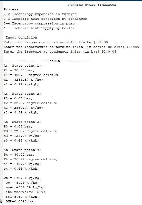
Result
output
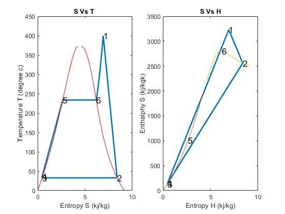
Graph
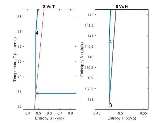
Zoom view for pump zone
1-2 temperature decreases
2-3 entropy decreases Temperature remain constant
3-4 entropy remains a constant temperature
4-1 Temperature and entropy increases
conclusion
Rankine cycle simulation is done using steam table function file using Matlab
Output as
net Work done
Wnet=667.79 kj/kg
thermal efficiency
`\eta=21.61%`
Back work ratio
BWR=0.0045
REFERENCES
https://www.e-education.psu.edu/eme812/node/708
https://lambdageeks.com/back-work-ratio/