Project 2 - Rankine cycle Simulator

Theory of Rankine Cycle

The Rankine cycle was named after him and describes the performance of steam turbine systems, though the theoretical principle also applies to reciprocating engines such as steam locomotives. The Rankine cycle is an idealized thermodynamic cycle of a constant pressure heat engine that converts part of heat into mechanical work. In this cycle, the heat is supplied externally to a closed loop, which usually uses water (in a liquid and vapor phase) as the working fluid. In contrast to the Brayton cycle, the working fluid in the Rankine cycle undergo the phase change from a liquid to vapor phase and vice versa.

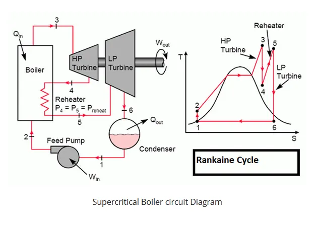
In an ideal Rankine cycle, the system executing the cycle undergoes a series of four processes: two isentropic (reversible adiabatic) processes alternated with two isobaric processes:

• Isentropic compression (compression in centrifugal pumps) – The liquid condensate is compressed adiabatically from state 1 to state 2 by centrifugal pumps (usually by condensate pumps and then by feedwater pumps). The liquid condensate is pumped from the condenser into the higher pressure boiler. In this process, the surroundings work on the fluid, increasing its enthalpy (h = u+pv) and compressing it (increasing its pressure). On the other hand, the entropy remains unchanged. The work required for the compressor is given by

• W_Pumps = H₂ – H₁.

• Isobaric heat addition (in a heat exchanger – boiler) – In this phase (between state 2 and state 3), there is a constant-pressure heat transfer to the liquid condensate from an external source since the chamber is open to flow in and out. The feedwater (secondary circuit) is heated to the boiling point (2 → 3a) of that fluid and then evaporated in the boiler (3a → 3). The net heat added is given by
• Q_add = H₃ – H₂
• Isentropic expansion (expansion in a steam turbine) – Steam from the boiler expands adiabatically from state 3 to state 4 in a steam turbine to produce work and then is discharged to the condenser (partially condensed). The steam works on the surroundings (blades of the turbine) and loses an amount of enthalpy equal to the work that leaves the system. The work done by the turbine is given by
• W_T = H₄ – H₃. Again the entropy remains unchanged.
• Isobaric heat rejection (in a heat exchanger) – In this phase, the cycle completes by a constant-pressure process in which heat is rejected from the partially condensed steam. There is heat transfer from the vapor to cooling water flowing in a cooling circuit. The vapor condenses, and the temperature of the cooling water increases. The net heat rejected is given by
• Q_re = H₄ – H₁
• 

• clear all
  close all
  clc
  %program for calculation of efficiency of rankine cycle
  %the rankine cycle follows this 4 process
  % 1-2 isentropic expansion in the turbine
  % 2-3 constant pressure heat rejection
  % 3-4 isentroic compression in the pump
  % 4-1 constant pressure heat addition by the boiler
  
  
  %turbine inlet temprature
  T1=400;
  %turbine inlet pressure
  p1=30;
  %turbine outlet pressure
  p2=0.05;
  
  %now we are going to take inputs from the Xsteam function
  % state point 1
  s1=XSteam('s_pT',p1,T1)
  h1=XSteam('h_pT',p1,T1)
  
  % state point 2
  
  T2=XSteam('Tsat_p',p2)
  T_sat=XSteam('Tsat_p',p1)
  s2=s1;
  sf2=XSteam('sL_p',p2)
  sg2=XSteam('sV_p',p2)
  hf2=XSteam('hL_p',p2)
  hg2=XSteam('hV_p',p2)
  x2=((s2-sf2)/(sg2-sf2));
  h2=hf2+(x2*(hg2-hf2))
  
  
  
  p3=p2;
  T3=T2;
  s3=XSteam('sL_p',p3)
  h3=XSteam('hL_p',p3)
  v3=XSteam('vL_p',p3)
  
  
  % state point 4
  s4=s3;
  p4=p1;
  cp4=XSteam('Cp_ps',p4,s4)
  cv4=XSteam('Cv_ps',p4,s4)
  g4=(cp4/cv4)
  o=(g4-1)/g4
  T4=T3*((p4/p3)^o)
  
  W_pump=v3*(p2-p1); %this will calculate work done by pump
  h4=h3+W_pump;
  
  %state point 5
  s5=XSteam('sL_p',p1)
  h5=XSteam('hL_p',p1)
  T5=XSteam('Tsat_p',p1)
  
  %state point 6
  s6=XSteam('sV_p',p1)
  h6=XSteam('hL_p',p1)
  T6=T5;
  
  %calculation
  W_turbine= h3-h4; %this will represents work done by tuebine
  
  
  W_net=W_turbine-W_pump;
  Qin=h1-h4;
  Qh=h3-h2;
  
  Efficiency=(W_net/Qin)*100;
  
  BWR= (W_pump/W_turbine); %BWR represent the back work ratio
  
  %ploting of T-S
  %plotting T_S Diagram
  t=linspace(5,400,50000) % here we have used linspace to take rrange bound calculation %with 50000 itration
  %now we are going to use for loop to plot the graph
  for i=1:length(t)
  s(i)=XSteam('sL_t',t(i));
  S(i)=XSteam('SV_t',t(i));
  h(i)=XSteam('hL_t',t(i));
  H(i)=XSteam('hV_t',t(i));
  end
  
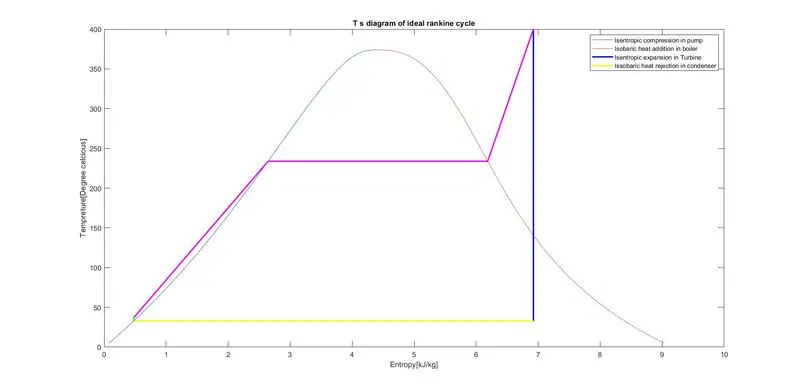
  figure(1)
  plot(s,t);
  hold on
  plot(S,t);
  
  plot([s1 s2],[T1 T2],'linewidth',2,'color','b')
  plot([s2 s3],[T2 T3],'linewidth',2,'color','y')
  plot([s3 s4],[T3 T4],'linewidth',2,'color','g')
  plot([s4 s5],[T4 T5],'linewidth',2,'color','m')
  plot([s5 s6],[T5 T6],'linewidth',2,'color','m')
  plot([s6 s1],[T6 T1],'linewidth',2,'color','m')
  xlabel('Entropy[kJ/kg]')
  ylabel('Tempreture[Degree celcious]')
  title('T s diagram of ideal rankine cycle')
  legend('Isentropic compression in pump','Isobaric heat addition in boiler','Isentropic expansion in Turbine','Issobaric heat rejection in condenser');
  %ploting of h-S
  %plotting h_S Diagram
  
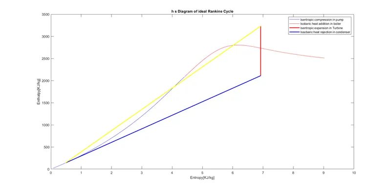
  figure(2)
  t=linspace(5,400,50000)
  for i=1:length(t)
  s(i)=XSteam('sL_t',t(i));
  S(i)=XSteam('sV_t',t(i));
  h(i)=XSteam('hL_t',t(i));
  H(i)=XSteam('hV_t',t(i));
  end
  plot(s,h,'color','b');
  
  hold on
  plot(S,H,'color','r');
  plot([s1 s2],[h1 h2],'linewidth',2,'color','r')
  plot([s2 s3],[h2 h3],'linewidth',2,'color','b')
  plot([s3 s4],[h3 h4],'linewidth',2,'color','g')
  plot([s4 s1],[h4 h1],'linewidth',2,'color','y')
  xlabel('Entropy[KJ/kg]')
  ylabel('Enthalpy[KJ/kg]')
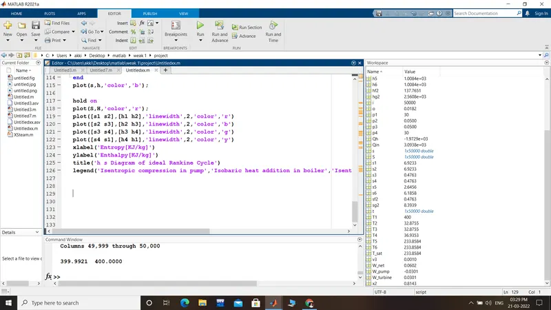
  title('h s Diagram of ideal Rankine Cycle')
  legend('Isentropic compression in pump','Isobaric heat addition in boiler','Isentropic expansion in Turbine','Issobaric heat rejection in condenser')
  
  

%all points how we got them

%we are using steam library to calculate the state points

%state point 1

%h1= enthalpy point 1 is Xsteam(h_pT,p1,T1) this means that from steam library search for the value of enthalpy at point p1 and t1.

%s1 = entropy at point1 (s_pT,p1,T1) this means that from steam library search for the value of entropy at point p1 and t1.

%hl1=saturated liquid enthalpy Xsteam(hL_p) this means that from steam library search for the value of enthalpy at point p1

%sg1=saturated vapour entropy Xsteam(sV_p) this means that from steam library search for the value of entropy at point p1

%T_sat1=saturated teprature Xsteam(Tsat_p) this means calculate the saturated temprature from steam library at p1 point

%hg1=saturated vapour enthalpy Xsteam(hV_p) this means that from steam library search for the value of enthalpy at point p1

%sl1=saturated liquid entropy Xsteam(sL_p) this means that from steam library search for the value of entropy at point p1

%state point 2

%s2=s1; here s1 is s2;

%sl2=Xsteam(sL_p,p2) this means that from steam library search for the value of entropy at point p2 in liquid state.

%sg2=Xsteam(sV_p,p2) this means that from the steam library search for the value of entropy at point p2 in vapour state.

%d= calculation of dryness fraction using formula

%hl2=Xsteam(hL_p,p2) this means that from steam library search for the value of enthalpy at point p2 in liquid state.

%hg2=Xsteam(hV_p,p2) this means from steam library search for the value of enthalpy at point p2 in vapour state

%h2=(hl2+ d*(hg2-hl2))

%T2=Xsteam(T_ph,p2,h2) calculate the temprature t2 form steam library using variable p2 nad h2

%Tsat2=saturated teprature Xsteam(Tsat_p) this means calculate the saturated temprature from steam library at p2 point

%state point 3

%h3=hl2

%s3=sl2

%p3=p2

%T3=T2

%state point 4

%s4=s3;

%p4=p1;

%h4=Xsteam(h_ps,p4,s4) calculate the enthalpy at point 4 from the steam library at p4 and s4 points

%T4=Xsteam(T_ps,p4,s4)calulate the temprature at point 4 from the steam library at point p4 and s4