Project 2 - Rankine cycle Simulator
AIM : Create a Rankine Cycle Simulator using OCTAVE/MATLAB.Your code should calculate the state points of the Rankine Cycle (any type of your choice) based on user inputs. Then, plot the corresponding T-s and h-s plots for the given set of inputs.
THEORY: The Rankine cycle is an idealized thermodynamic cycle describing the process by which certain heat engine such as steam turbine or reciprocating steam engines, allow mechanical work to be extracted from a fluid as it moves between a heat source and heat sink.
There are four processes in the Rankine cycle:
Process 1–2: The working fluid is pumped from low to high pressure. As the fluid is a liquid at this stage, the pump requires little input energy. Process 1-2 is isentropic compression.
Process 2–3: The high-pressure liquid enters a boiler, where it is heated at constant pressure by an external heat source to become a dry saturated vapour. The input energy required can be easily calculated graphically, using an enthalpy–entropy chart (h–s chart, or Mollier diagram), or numerically, using steam tables or software. Process 2-3 is constant pressure heat addition in boiler.
Process 3–4: The dry saturated vapour expands through a turbine, generating power. This decreases the temperature and pressure of the vapour, and some condensation may occur. The output in this process can be easily calculated using the chart or tables noted above. Process 3-4 is isentropic expansion.
Process 4–1: The wet vapour then enters a condenser, where it is condensed at a constant pressure to become a saturated liquid. Process 4-1 is constant pressure heat rejection in condenser.
RANKINE CYCLE EFFICIENCY:

BACK WORK RATIO:
BW RATIO = Wp/Wt
PROGRAM:
% programming for rankine cycle simulator
clear all
close all
clc
disp(' RANKINE CYCLE ');
disp('1-2 is constant pressure heat addition in the boiler');
disp('2-3 is isentropic expantion in the turbine');
disp('3-4 is constant pressure heat removal in the condenser');
disp('4-1 isentropic compression in the pump');
p1 = input('nvalue of pressure at turbine inlet ,p1 (inbar) = ');
T1 = input('nvalue of temperature at turbine inlet, T1(in degree) = ');
p2 = input('nvalue of pressure at condenser inlet, p2(in bar) = ');
% At state 1
h1 = XSteam('h_pT', p1, T1);
s1 = XSteam('s_pT', p1, T1);
% At state 2
s2 = s1;
sf2 = XSteam('sL_p',p2);
sg2 = XSteam('sV_p',p2);
x2 = (s2-sf2)/(sg2-sf2);
hf2 = XSteam('hL_p',p2);
hg2 = XSteam('hV_p',p2);
h2 = hf2+ (x2*(hg2-hf2));
% At state 3
p3 = p2;
s3 = XSteam('sL_p', p3);
h3 = XSteam('hL_p', p3);
% At state 4
s4 = s3;
p4 = p1;
% Work done by the turbine
Wt = h1 - h2;
%Work done to run pump
v3 = XSteam ('vL_p',p3);
Wp = v3*(p4 - p3)*100;
h4 = h3 + Wp;
%Net Work
Wnet = Wt -Wp;
%Heat in to the system
Qin = h1-h4;
%Heat out to the system
Qout = h2 - h3;
%Thermal efficiency
thermal_effi = (Wnet/Qin)*100
%Specific steam consumption
%SSC = mass flow rate/power
SSC = (3600/ Wnet);
% Back Work ratio
BW = (Wp/Wt)
% calculation of Temperatures at the state points
T3 = XSteam('Tsat_p', p3);
T2 = T3;
Cp4 = XSteam('cp_ps',p4, s4);
Cv4 = XSteam('cv_ps',p4, s4);
k = Cp4/Cv4
T4 = T3/((p3/p4)^((k-1)/k));
% calculating temperature, entropy and enthalpy at the vapour and liquid line for plotting
T6 = XSteam('Tsat_p', p1);
s5 = XSteam('sL_p', p1);
s6 = XSteam('sV_p', p1);
h5 = XSteam('hL_P', p1);
h6 = XSteam('hV_p', p1);
T5 = T6;
%plotting the saturation curve
T = linspace(1,375,1000);
for i=1:length(T)
sf(i) = XSteam('sL_T', T(i));
sg(i) = XSteam('sV_T', T(i));
hf(i) = XSteam('hL_T', T(i));
hg(i) = XSteam('hV_T', T(i));
end
%plotting T-s diagram
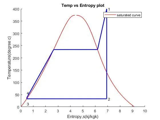
figure(1)
hold on
plot(sf, T, 'r','linewidth',1)
plot(sg, T, 'r','linewidth',1)
plot([s1 s2],[T1 T2],'b','linewidth',2)
plot([s2 s3],[T2 T3],'b','linewidth',2)
plot([s3 s4],[T3 T4],'b','linewidth',2)
plot([s4 s5],[T4 T5],'b','linewidth',2)
plot([s5 s6],[T5 T6],'b','linewidth',2)
plot([s6 s1],[T6 T1],'b','linewidth',2)
sc1 = linspace(s6, s1, 1000);
for j = 1:length(sc1)
Tc(i) = XSteam('T_ps', p1, sc1(j));
end
% plot(sc1, Tc, 'b','linewidth',2)
text(s1+0.1, T1, '1')
text(s2+0.1, T2, '2')
text(s3, T3-20, '3')
text(s4, T4+20, '4')
title('Temp vs Entropy plot')
xlabel('Entropy,s(kj/kgk)' )
ylabel('Temperature(degree c)')
legend('saturated curve')
%plotting h-s diagram
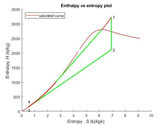
figure(2)
hold on
plot(sf, hf, 'r','linewidth',1)
plot(sg, hg, 'r','linewidth',1)
plot([s1 s2],[h1 h2],'g','linewidth',2)
plot([s2 s3],[h2 h3],'g','linewidth',2)
plot([s3 s4],[h3 h4],'g','linewidth',2)
hc = linspace(h4, h5, 100);
for r = 1:length(hc)
sch(r) = XSteam('s_ph', p1, hc(r));
end
plot(sch,hc, 'r', 'linewidth', 2)
plot([s5 s6],[h5 h6],'g','linewidth',2)
for m = 1:length(sc1)
hc1(m) = XSteam('h_ps', p1, sc1(m));
end
plot(sc1, hc1, 'r', 'linewidth', 2 )
text(s1+0.1, h1,'1')
text(s2+0.1, h2,'2')
text(s3, h3-100, '3')
text(s4, h4 +200, '4')
title('Enthalpy vs entropy plot')
xlabel('Entropy , S (kj/kgk) ')
ylabel('Enthalpy, H (kj/kg) ')
legend('saturated curve','location','northwest')
% for the results which is apper in the command window
disp('results')
p1 = p1;
T1 = T1;
p2 = p2;
disp('At stage point 1');
n1 = sprintf('p1 is %.3f bar',p1);
disp(n1);
n2 = sprintf('T1 is %.3f c',T1);
disp(n2);
n3 = sprintf('h1 is %.3f kj/kg',h1);
disp(n3);
n4 = sprintf('s1is%.3f kj/kgk',s1);
disp(n4);
disp('at stage point 2');
n11 = sprintf('p2 is %.3f bar',p2);
disp(n11);
n21 = sprintf('T2 is %.3f c',T2);
disp(n21);
n31 = sprintf('h2 is%.3f kj/kg',h2);
disp(n31);
n41 = sprintf('s2 is %.3f kj/kgk',s2);
disp(41);
disp('at stage point 3');
n12 = sprintf('p3 is %.3f bar',p3);
disp(n12);
n22 = sprintf('T3 is %.3f c',T3);
disp(n22);
n32 = sprintf('h3 is %.3f kj/kg',h3);
disp(32);
n42 = sprintf('s3 is %.3f kj/kgk',s3);
disp(42);
disp('at stage point 4');
n13 = sprintf('p4 is %.3f bar',p4);
disp(n13);
n23 = sprintf('T4 is %.3f c',T4);
disp(n23);
n33 = sprintf('h4 is %.3f kj/kg',h4);
disp(n33);
n43 = sprintf('s4 is %.3f kj/kgk',s4);
disp(n43);
n14 = sprintf('Wt is%.3f kj/kg',Wt);
disp(n14);
n15 = sprintf('Wp is %.3f kj/kg',Wp);
disp(n15);
n16 = sprintf('Wnet is %.3f kj/kg',Wnet);
disp(n16);
n17 = sprintf('Thermal_efficiency is %.2f percent',thermal_effi);
disp(n17);
n18 = sprintf('SSC is %.2f kg/kWh',SSC);
disp(n18);
n19 = sprintf('Back work ratio is %.3f ',BW);
disp(n19);
EXPLINATION :
In this program first we give the four stages of rankine cycle then given the inputs of T1,P1,P2.
Then we give the equations from the given data of Xsteam for stage 1, stage 2, stage 3 and stage 4.
After that we fid out the equations for workdone for turbine and runpump then network heat in to the system and heat out to the system and rhermal efficiency.
Then we introduce equations for SSC which is called as specific heat consumption and back work ratio.
Calculate the temperatures at each points and calculate the vapour and liquid line plotting for temperature , entropy, enthalpy .
Plotting the saturated curve T(linspace) and in the for loop sf, sg, hf are introduced.
Saturated curve is plotted in green for saturated liquid and saturated gases in T-S and H-S it is black.
Plot of Tvs S and Hvs S is created for all the points obtained from the program using plot command mention the label, linewidth, color and title.
The plot changes as the user input for the above mention inputs.
Results are displayed in command windows by using sprintf command.
OUTPUT COMMAND WINDOW RESULTS
RANKINE CYCLE
1-2 is constant pressure heat addition in the boiler
2-3 is isentropic expantion in the turbine
3-4 is constant pressure heat removal in the condenser
4-1 isentropic compression in the pump
nvalue of pressure at turbine inlet ,p1 (inbar) = 30
nvalue of temperature at turbine inlet, T1(in degree) = 400
nvalue of pressure at condenser inlet, p2(in bar) = 0.05
thermal_effi =
36.1671
BW =
0.0027
k =
1.0185
results
At stage point 1
p1 is 30.000 bar
T1 is 400.000 c
h1 is 3231.571 kj/kg
s1is6.923 kj/kgk
at stage point 2
p2 is 0.050 bar
T2 is 32.875 c
h2 is2110.708 kj/kg
41
at stage point 3
p3 is 0.050 bar
T3 is 32.875 c
32
42
at stage point 4
p4 is 30.000 bar
T4 is 36.935 c
h4 is 140.776 kj/kg
s4 is 0.476 kj/kgk
Wt is1120.863 kj/kg
Wp is 3.011 kj/kg
Wnet is 1117.852 kj/kg
Thermal_efficiency is 36.17 percent
SSC is 3.22 kg/kWh
Back work ratio is 0.003
>>
GRAPH RESULTS: