Project 2 - Rankine cycle Simulator

Aim -

• Create a Rankine Cycle Simulator using OCTAVE/MATLAB.
• 

close all
clear all
clc

%Dispalying
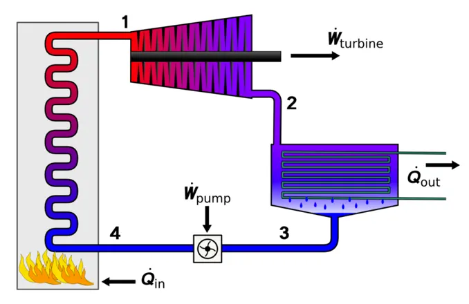
disp('RANKINE CYCLE SIMULATOR')

disp('1-2 Isentropic Expansion in turbine')
disp('2-3 Const pressure Heat rejectionby the codensar')
disp('3-4 Isentropic compression in the pump')
disp('4-1 Const pressure Heat addition by the boiler')


%RANKINE CYCLE
%Inputs
p1=input('nValue of pressure at turbine inlet,p1(in bar)=');
t1 = input('nValue of temperature at turbine inlet, t1(in degree.C)=');
p2= input('nValue of temperature at condenser inlet,p2(in bar)=');


%state point 1
s1=XSteam('s_pt', p1,t1);
h1=XSteam('h_pt', p1 ,t1);

%state point 2
s2=s1;
sf2=XSteam('sL_P',p2);
sg2=XSteam('sV_P',p2);
hf2=XSteam('hL_P',p2);
hg2=XSteam('hV_P',p2);
x2=((s2-sf2)/(sg2-sf2));
h2=hf2+(x2*(hg2-hf2));

%state point 3
p3=p2;
s3=XSteam('sL_P',p3);
h3=XSteam('hL_P',p3);

%state point 4
s4=s3;
p4=p1;
v3=XSteam('vL_P',p3);
wp= v3*(p4-p3)*100;
h4 = h3 +wp;

%turbine work
wt=h1-h2;

%WORK NET
Wnet=wt-wp;
 
% Heat added
Qin=h1-h4;

% Heat rejected
Qout=h2-h3;

% Theramal Efficiency
N=Wnet/Qin;

%steam consumption
SSC=(3600/Wnet);

%TEMPERATURES AT VARIES POINT
t3=XSteam('tsat_p',p3);
t2=t3;
Cp4=XSteam('Cp_ps',p4,s4);
Cv4=XSteam('Cv_ps',p4,s4);
k=Cp4/Cv4;
t4=t3/((p3/p4))^((k-1/k));
t6=XSteam('tsat_p',p1);
t5=t6;
s5=XSteam('sL_P', p1);
s6=XSteam('sV_P',p1);
h5=XSteam('sL_P',p1);
h6=XSteam('hV_P',p1);

t=linspace(1,375,1000);
for i = 1:length(t)
     sf(i)= XSteam('sL_T',t(i));
    sg(i)= XSteam('sV_T',t(i));
    hf(i)= XSteam('hL_T',t(i));
    hg(i)= XSteam('hV_T',t(i));
end

%PLOTING
figure(1)
hold on
plot(sf,t ,'r',LineWidth=1)
plot(sg,t,'r',LineWidth=1)
plot([s1 s2],[t1,t2],LineWidth=2)
plot([s2 s3],[t2 t3],LineWidth=2)
plot([s3 s4], [t3 t4],LineWidth=2)
plot([s4 s5],[t4 t5],LineWidth=2)
plot([s5 s6],[t5 t6],LineWidth=2)

sc1=linspace(s6,s1,1000);

for l =1:length(sc1)
    Tc1(l)=XSteam('T_ps',p1, sc1(l));
end
plot(sc1, Tc1,LineWidth=2)
text(s1,t1,'1')
text(s2,t2,'2')
text(s3,t3,'3')
text(s4,t4,'4')
title('entrophy vs temperature')
xlabel('entrophy')
ylabel('temperature')

%PLOTING enthalhy vs Entropy
figure(2)
hold on
plot(sf,hf,'r',LineWidth=1)
plot(sg,hg,'r',LineWidth=1)
plot([s1 s2],[h1 h2], 'k', 'LineWidth',2)
plot([s2 s3], [h2 h3],'k', 'linewidth',2)
plot([s3 s4], [h3 h4],'k', 'linewidth',2)
plot([s4 s1], [h4 h1],"k", 'linewidth',2)
hc=linspace(h4, h5 ,100);
for k =1:length(hc)
sch(k)= XSteam('s_ph', p1 , hc(k));
end
text(s1,h1,'1')
text(s2,h2,'2')
text(s3,h3,'3')
text(s4,h4,'4')
title('Enthalphy vs Entrophy plot')
xlabel('Entrophy,S(kj/kgk)')
ylabel('Enthalphy, H(KJ/KG)')


%dispalying result
disp('RESULT');
fprintf('At state point 1''\n')
fprintf('p1 = %10f in bar    ', p1);
fprintf('t1 =  %11f in deg.C   ', t1);
fprintf('h1= %12f in kj/kg   ',h1);
fprintf('s1=%9f in kj/kg-k   ''\n',s1);

fprintf('At state point 2n''\n')
fprintf('p2 = %10f in bar    ',p2 );
fprintf('t2= %11f in deg.C     ',t2);
fprintf('h2= %12f in kj/jg    ',h2);
fprintf('s2=%9f in kj/kg-kn''\n',s2);


fprintf('At state point 3''\n')
fprintf('p3= %10f in bar    ', p3);
fprintf('t3= %11f in deg.C      ',t3);
fprintf('h3= %12f in kj/jg  ',h3);
fprintf('s3=%9f in kj/kg-k   ''\n',s3);




fprintf('At state point''\n')
fprintf('p4 = %10f in bar  ',p4 );
fprintf('t4= %11f in deg.C       ',t4);
fprintf('h4= %12f in kj/jg  ',h4);
fprintf('s4=%9f in kj/kg-k  ''\n',s4);

disp('Turbine work')
fprintf('wt= %10f in kg/kgn''\n', wt)

disp('Net Work')
fprintf('Wnet= %10f in kj/kgn''\n',Wnet)

disp('steam consumption')
fprintf('ssc= %10f in k''\n',SSC)



disp('Thermal Efficiency')
fprintf('N= %10f in percentn''\n',N)

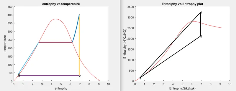
PLOTS:-

[T VS H],[H VS S]

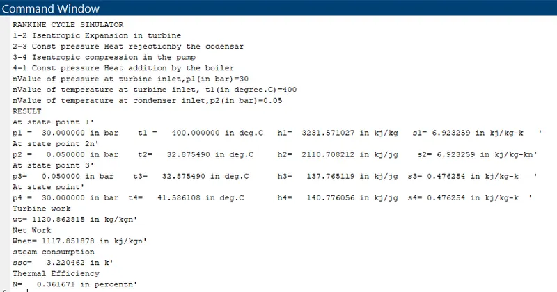
RESULTS :-

Explanation:-

1.)Xsteam data is used to extract the different properties of steam and water for e.g enthalpy entropy temperature pressure etc.

2). with help of inlets data and Xsteam data, the program calculates all state points of rankine cycle.

3). The Xsteam data works as :

S1=xsteam('s_pt', p1 ,t1);

4). saturation curve is plotted in red for saturated liquid and saturated gas.

5). Plot of TVs s and h vs s is created from all the points obtained from program.

6).The plot changes as the user inputs changes for the above mentioned inputs.

7). Results are displayed in the command window.