Project 2 - Rankine cycle Simulator

AIM:-

1) to simulate a rankie cycle using matlab

2)extracting steam and water properites from Xstrsm files

3)calculating all the state points of the cycle and to plot T vs S and H vs S.

Theory:-

The Rankine cycle was named after him and describes the performance of steam turbine systems, though the theoretical principle also applies to reciprocating engines such as steam locomotives. In general, the Rankine cycle is an idealized thermodynamic cycle of a constant pressure heat engine that converts part of heat into mechanical work. In this cycle the heat is supplied externally to a closed loop, which usually uses water (in a liquid and vapor phase) as the working fluid. In contrast to the braytom, the working fluid in the Rankine cycle undergo the phase change from a liquid to vapor phase and vice versa.

While many substances could be used as the working fluid in the Rankine cycle (inorganic or even organic), water is usually the fluid of choice due to its favorable properties, such as its non-toxic and unreactive chemistry, abundance, and low cost, as well as its thermodynamic properties. For example, water has the highest specific heat of any common substance – 4.19 kJ/kg K. Moreover it has very high , which makes it an effective coolant and medium in thermal power plants and other energy industry. In case of the Rankine cycle, almost cannot be used (steam do not follow pV=nRT), therefore all important parameters of water and steam are tabulated in so called steam tables

One of the major advantages of the Rankine cycle is that the compression process in the pump takes place on a liquid. By condensing the working steam to a liquid (inside a condenser) the pressure at the turbine outlet is lowered and the energy required by the feed pump consumes only 1% to 3% of the turbine output power and these factors contribute to a higher efficiency for the cycle.

In an ideal Rankine cycle, the system executing the cycle undergoes a series of four processes: two isentropic (reversible adiabatic) processes alternated with two isobaric processes,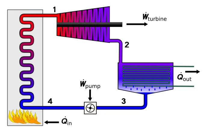

PROGRAM:-

clear all 
close all

dispt RANKINE CYCLE):

dispt 1-2 is constant pressure heat addition in the boiler);

disp('2-3 is Isentropic Expansion in the Turbine');

disp ('3-4 is constant pressure hest removal in the Condenser'):

disp('4-1 is Isentropis compression in the purp);

pt input('Value of pressure at turbine inlet, plin bar)");

11 input('nvalue of temperature at turbine inlet, Ticin degree.C));

p2= Input('nValue of pressure at condenser inlet, p2cin bar) = 3;


At State 1

s Extracting Enthalpy at state pt 1

% Similarly

Tsentropic Expansion:

s saturated Liquid Entropy % Saturated Vapour Entropy

At State 2

s1 = s2;

sf2 xstean("st_p¹, p2);

sg2= X5team SV_p, p2)

x2 = (2-st2)/(sg2-st21:

hf2=x5team'hi p. p2):

hg2=x5teamt V_P, p2); 
h2 hf2 (x2*(hg2-2));

SAt State 3

hd stean('hL_P¹, 03):

At State 4

34 - 13: p4 = pt;

s work done by turbine wth1 h2:

work done to run pump v3 XStean(VL p. p3):

wpv3 (p4-p3j 100;

Net work wnet Wt Mp;

Seat into the syste system

SHeat out of the system Qout 12 h;

SThermal efficiency

thermal eff (whet/Qin) 1001

Specific Stem Consumption

NSSC mass flow rate/power

* Constant pressure Heat rejection in Condenser

s Back Work ratio

BW (W/W)

s Calculation of Temperatures at the state points T3 XStean(That p.p3);

12= 13:

Cp4 =XSteam('Cp_ps, p4, 34');

Cv4 =xSteam ('Cy_ps, p4, 34');

k = C₂4/CV4;

14 13/([p3/p4)^((k-11/k3);
T6 XSteam('Tsat_p', p1);

s5 = XSteam('sl_p', p1);

s6 = XSteam('sV_p', p1);

h5 XSteam('hL_p', p1);

h6 XSteam (¹hV_p¹, p1);

T5 = 16;

18

% Plotting the saturation curve T = linspace(1,375,1000);

for i=1:length(T)

sf(i)= XSteam('sL_T', T(1));

sg(i) = XSteam('sV_T', T(i));

hf(1) = XSteam ('hL_T', T(i));

hg(i)= XSteam('hV_T', T(i));

end

%Plotting T-s diagram

figure (1)

hold on

plot(sf, T, 'r', 'linewidth',1) plot(sg, T, 'r', 'linewidth',1)

plot([s1 s2], [T1 T2], 'b', 'linewidth', 2)

plot([s2 s3], [T2 T3], 'b', 'linewidth', 2)

plot([s3 s4], [T3 T4], 'b', 'linewidth', 2)

plot([s4 s5], [T4 T5], 'b', 'linewidth', 2) plot([s5 s6], [T5 T6], 'b', 'linewidth', 2)

sc1=linspace(s6, s1, 1000);

for 1 1:length(sc1) Tc1(1) = XSteam ('T_ps', p1, sc1(1));

end plot(sc1, Tc1, 'b', 'linewidth', 2)

text(s1+0.1, T1, '1') text(s2+0.1, T2, '2')

text(s3, T3-20, '3')

text(s4, T4+20, '4')

title('Temp vs Entropy plot')

xlabel('Entropy ,S (Kj/kgk') ylabel('Temperature (degree () ¹)

legend('Saturation curve')

%Plotting h-s diagram

figure (2)

hold on

plot(sf, hf, 'k', 'linewidth', 1) plot(sg, hg. 'k', linewidth", 1)

plot([s1 s2], [h1 h2], 'r', 'linewidth', 2)

plot([s2 s3], [h2 h3], 'r', 'linewidth', 2)

plot([s3 s4], [h3 h4], 'r', 'linewidth', 2)

hc linspace(h4, h5, 100);

for r=1:length(hc)

sch(r) = XSteam('s_ph', p1, hc(r));

end

plot(sch, hc, 'r', 'linewidth', 2) plot([s5 s6], [h5 h6], 'r', 'linewidth', 2)

for m=1:length(sc1))

hc1(m) end

XSteam('h_ps', p1, sc1(m));

plot(sc1, hc1, 'r', 'linewidth', 2). text(s1+0.1, h1, '1')

text(s2+0.1, h2, '2') text(s3. h3-100, '3')

text(s4, h4 +200, '4')

title('Enthalpy vs Entropy plot')

xlabel('Entropy, 5 (KJ/kgk) ').

ylabel('Enthalpy, H (KJ/kg)')

legend('Saturation curve', 'location', 'northwest')

% Displaying the Results in the Command Window:

disp('Results');

p1 = p1; I1 = 11:

p2 = p2;
% Displaying the Results in the Command Window:

disp('Results');

p1 = p1;

11 = I1 p2 = p2;

disp('At stage point 1'); n1 sprintf('P1 is %.3f bar',p1);

disp(nl); n2 sprintf('T1 is %.3f C¹, T1);

disp(n2); n3 sprintf('h1 is %.3f kJ/kg,h1);

disp(n3); n4 = sprintf('s1 is %.3f kJ/kgK',s1);

disp(n4);

disp('At stage point 2'); n11 sprintf('P2 is %.3f bar',p2);

disp(n11); n21 sprintf('T2 is %.3f C',T2);

disp(n21);

n31 = sprintf('h2 is %.3f kJ/kg',h2);

disp(n31);

n41 sprintf('s2 is %.3f kJ/kgk',s2); 
disp(n41);

disp('At stage point 3'); n12 sprintf('P3 is %.3f bar¹,p3);

disp(n12);

n22 = sprintf('T3 is %.3f C',T3); n32 sprintf('h3 is %.3f kJ/kg',h3);

disp(n22);

disp(n32); n42 sprintf('s3 is %.3f kJ/kgK',s3);

disp(n42);

disp('At stage point 4');

n13 sprintf('P4 is %.3f bar',p4);

disp(n13);

n23 = sprintf('T4 is %.3f C',T4);

disp(n23);

n33 sprintf('h4 is %.3f kJ/kg',h4);

disp(n33);

n43 = sprintf('s4 is %.3f kJ/kgk', s4); disp(n43);

n14 sprintf('Wt is %.3f kJ/kg',Wt);

disp(n14):

n15 sprintf('Wp is %.3f kJ/kg',Wp);

disp(n15);

n16 sprintf('Whet is %.3f kJ/kg,Wnet);

disp(n16);

n17 sprintf('Thermal_efficiency is %.2f Percent', thermal_eff);

disp(n17);

n18 sprintf('SSC is %.2f kg/kWh,SSC);

disp(n18);

n19 sprintf('Back work ratio is %.3f, BW); 
disp(n19);