Project 2 - Rankine cycle Simulator

# RANKINE CYCLE

OBJECTIVE:

1. To simulate rankine cycle using mathlab.
2. extracting steam and water properties from XSteam data (IAPWS IF - 97 standard)
3. caculating all the state points based on user inputs.
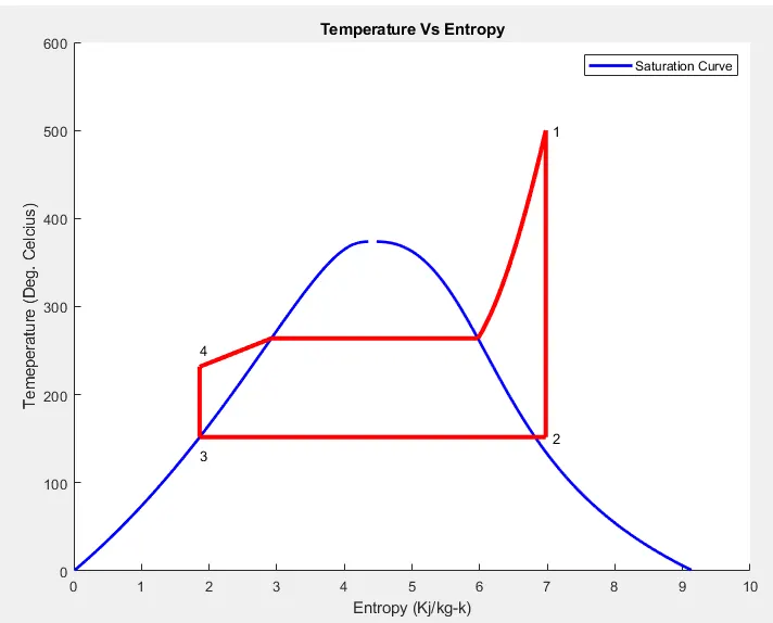
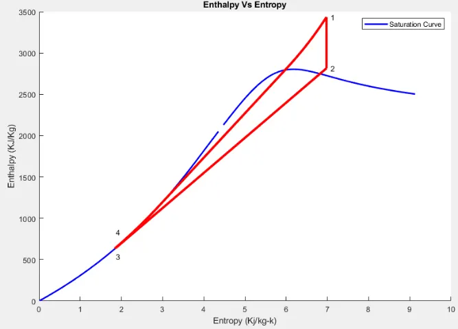
4. plotting the T vs s and H vs s plot.

RANKINE CYCLE:

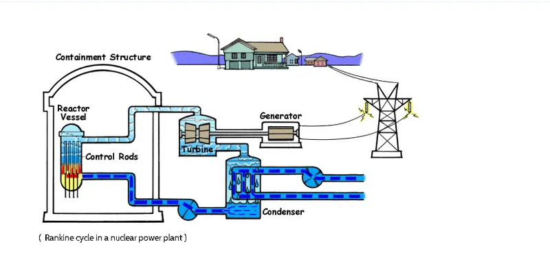
Rankine cycle is an idealized thermodynamic cycle or heat engine which fuel mis used to produce heat with in boiler.

1. In this project an idealized cycle is simulated.
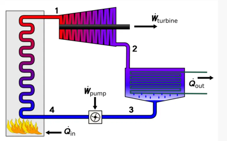
2. rankine cycle is delivered out of carnot cycle.its power depends on the temperature diff between heat source and cold source.
3. efficiency of rankine cycle is limited by high heat of vaporation of working fluid.

PROCESSES AND WORKING:

There are four process in rankine cycle,

1. Process 1-2: Isoentropic expansion in the turbine.
2. Process 2-3: constant pressure heat rejection in condensor.
3. Process 3-4: Isentropic compresion on the pump.
4. Process 4-1: constant pressure heat addition in the boiler.

PROJECT PROGRAM:

% Rankine_cycle project
clear all
close all
clc

% printing introduction
fprintf('RANKINE CYCLE SIMULATOR \n')
fprintf('\n1-2 is isentropic expansion in the Turbine \n')
fprintf('2-3 is Constant Pressure Heat Rejection by the Condenser \n')
fprintf('3-4 is isentropic compression in pump \n')
fprintf('4-1 is Constant Pressure Heat Addition by the Boiler \n')

% obtaining input data
p1 = input('\nValue of Pressure at the Turbine Inlet(in bar): ');
t1 = input('Value of Temperature at the Turbine Inlet(in Degree Celcius): ');
p2 = input('Value of Pressure at Turbine Outlet (in bar): ');

% Extracting data_defining varibles
% state 1
h1 = XSteam('h_pt',p1,t1);  % Enthalpy
s1 = XSteam('s_pt',p1,t1);  % Entropy

% state 2
s2 = s1;
sf2 = XSteam('sL_p',p2);   
Sg2 = XSteam('sV_P',p2);
x2 = ((s2-sf2)/(sg2-sf2));
hf2 = XSteam('hL_p',p2);
hg2 = XSteam('hV_p',p2);
h2 = hf2 +(x2*(hg2-hf2));


% state 3
p3 = p2;
s3 = XSteam('sL_p',p3);
h3 = XSteam('hL_p',p3);

% state 4
s4 = s3;
P4 = p1;

% turbine work
Wt = h1-h2;

% work done by run the pump
v3 = XSteam('vL_p',p3);
Wp = v3*(p4 - p3)*100;
h4 = h3 + Wp;

% Net work
Wnet = Wt-Wp;


% Heat addition
Qin = h1 - h4;

% Heat rejection
Qout = h2-h3;

% thermal efficiency
eff = (Wnet/Qin)*100;

% specific steam consuption
% SSC = mass flow rate/power
SSC = 3600/Wnet;

% calculation temperature at the state point
t3 = XSteam('tsat_p',p3);
t2 = t3;
Cp4 = XSteam('Cp_ps',p4,s4);
Cv4 = XSteam('Cv_ps',p4,s4);
k = Cp4/Cv4;
t4 = t3/((p3/p4)^((k-1)/k));

% calculation temperature, entropy and enthalpy at the vapour and liquid
t6 = XSteam('tsat_p', p1);
s5 = XSteam('sL_p', p1);
s6 = XSteam('sV_p', p1);
h5 = XSteam('hL_p', p1);
h6 = XSteam('hL_p', p1);
t5 = XSteam('hV_p', p1);

% plotting the saturation curve
T = linspace(1,375,1000);
for i =1:length(t)
    
    sf(i) = XSteam('sL_t', T(i));
    sg(i) = XSteam('sv_t', T(i));
    hf(i) = XSteam('hL_t', T(i));
    hg(i) = XSteam('hV_t', T(i));

end


% plotting T-s diagram
figure(1)
hold on
plot(sf,t, 'r','linewidth',1)
plot(sg,t, 'r','linewidth',1)
plot([s1 s2], [T1,T2], 'k', 'linewidth', 2)
plot([s2 s3], [T2,T3], 'k', 'linewidth', 2)
plot([s3 s4], [T3,T4], 'k', 'linewidth', 2)
plot([s4 s5], [T4,T5], 'k', 'linewidth', 2)
plot([s5 s6], [T5,T6], 'k', 'linewidth', 2)
scl = linspace(s6, s1, 1000);
for l = 1:length(scl)
    tcl(l) = XSteam('t_ps',p1, sc1(1));
    
end
plot(sc1, tc1, 'k', 'linewidth', 2)
text(s1+0.1, T1, '1')
text(s2+0.1, T2, '1')
text(s3, t3-20, '1')
text(s4, t4+20, '1')
title('Temp vs Entropy plot')
xlabel('Entropy ,s (kj/kgk')
ylabel('Temperature (degree c) ')
legend('saturation curve')


% plotting h-s diagram
figure(2)
hold on
plot(sf, hf, 'r','linewidth',1)
plot(sg, hg, 'r','linewidth',1)
plot([s1 s2], [h1,h2], 'k', 'linewidth', 2)
plot([s2 s3], [h2,h3], 'k', 'linewidth', 2)
plot([s3 s4], [h3,h4], 'k', 'linewidth', 2)
hc = linspace(h4, h5, 100);
for k = 1:length(hc)
    sch(k) = XSteam('s_ph',p1, hc(k));
    
end
plot(sch,hc, 'k', 'linewidth',2)
plot([s5 s6], [h5 h6], 'k', 'linewidth', 2)
for m = 1:length(sc1)
    hc1(m) = XSteam('h_ps', p1, sc1(m));
end
plot(sc1,hc1, 'k', 'linewidth', 2)
text(s1+0.1, h1, '1')
text(s2+0.1, h2, '2')
text(s3, h3-100, '3')
text(s4, h4 +200, '4')
title('Enthalpy vs Entropy plot')
xlabel('Entropy, S (kj/kgk)')
ylabel('enthalpy, H (kj/kg)')
legend('saturation curve','location','northwest')



% displaying result
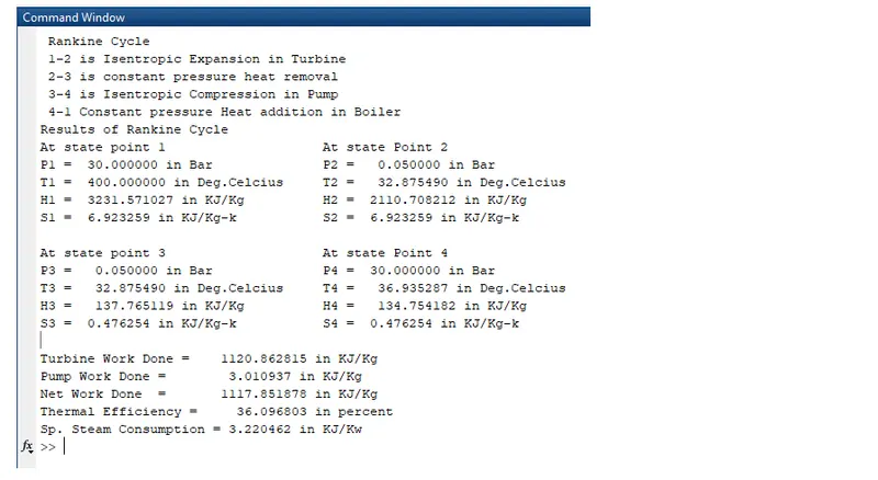
disp(' RESULTS');
fprintf('At state point 1:n');
fprintf('p1: %8.3f bar', p1);
fprintf('T1: %8.3f Cn', T1);
fprintf('h1: %8.3f KJ/Kg\n', h1);
fprintf('s1: %8.3f KJ/Kg-Knn', s1);

fprintf('nAt state point 2:n');
fprintf('p2: %8.3f barn', p2);
fprintf('T2: %8.3 Cn', T2);
fprintf('h2: %8.3f KJ/Kgn', h2);
fprintf('s2: %8.3f KJ/Kg-Kn', s2);
fprintf('x2: %8.3fnn', x2);

fprintf('At state point 3:n');
fprintf('p3: %8.3f barn', p3);
fprintf('T3: %8.3f Kn', T3);
fprintf('h3: %8.3f KJ/Kgn', h3);
fprintf('s3: %8.3f KJ/Kg-Kn', s3);

fprintf('At state point 4:n');
fprintf('p4: %8.3f barn', p4);
fprintf('T4: %8.3f Kn', T4);
fprintf('h4: %8.3f KJ/Kgn', h4);
fprintf('s4: %8.3f KJ/Kg-Kn', s4);

fprintf('Turbine Work: %8.3f KJ/Kgn', Wt);
fprintf('Pump Work: %8.3f KJ/Kgn', Wp);
fprintf('Wnet: %8.3f KJ/Kg-Kn', Wnet)
fprintf('Efficiency: %8.3f percent n', eff);
fprintf('S.S.C: %8.3f Kg/Kwhn', SSC);

• XSteam data is used to extract steam and water properties of enthalpy. entropy pressure and Temperature for sat liquid ,sat vapour condition.
• The program requires the input of pressure (in bar) at state point 1(turbine inlet), temperature at same point (deg celcius).
• h1 = XSteam('hP_t',p1,t1) returns the enthalpy of water at given pressure and temperature.
• As we extract the data we use the thermodynamic relation.
• Sf and sg ,hf and hg where f and g stand for saturated liquid and saturated vapour respectively.
• eff and specfic heat consumption (SSC).
• result are displayed.

[Tvs S] & [H vs S] PLOT:

COMMAND WINDOW:

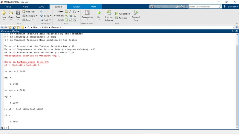
ERROR: