Project 2 - Rankine cycle Simulator

RANKING CYCLE SIMULATOR

AIM :

• The concept of Rankine cycle by referring to standard thermal engineering text book.

OBJECTIVES :

• calculate the state points of the Rankine Cycle based on user inputs.
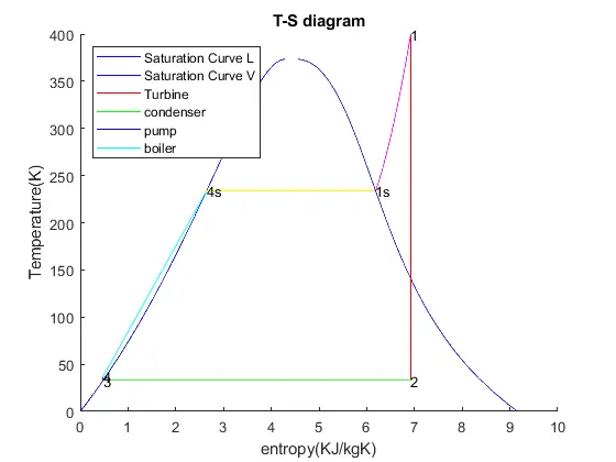
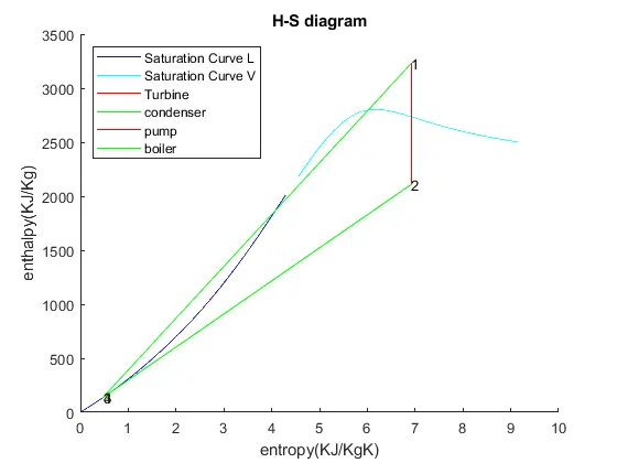
• Then, plot the corresponding T-s and h-s plots for the given set of inputs. Title and axes labels are a must, while legends could be used if necessary.
• Attach a report explaining the working of a rankine cycle simulator and also the research done by you.

THEORY:

• The Rankine cycle is an idealized thermodynamic cycle of a heat engine that converts heat into mechanical work while undergoing a phase change.
• It is an idealized cycle in which friction losses in each of the four components are neglected.
• The heat is supplied externally to a closed loop, which usually uses water as the working fluid.

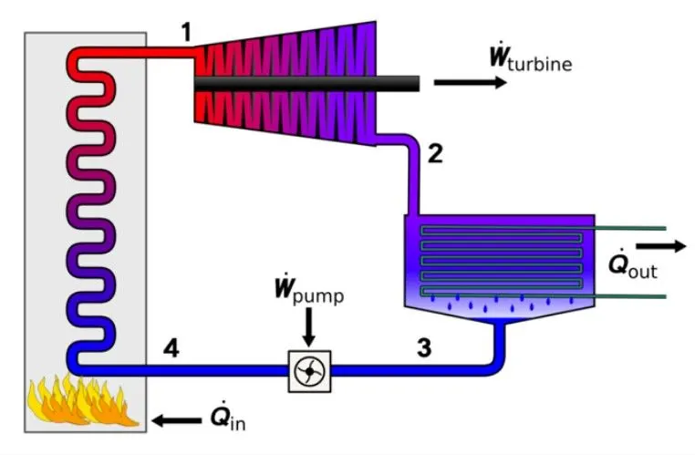
Four components of the Rankine cycle:

1. Pump
2. Boiler
3. Turbine
4. Condenser

Four processes of the Rankine cycle:

1-2: Isentropic Expansion

• Turbine (1-2): Superheated steam enters into the Turbine and expands isentropically resulting in the production of work.
• The shaft of the turbine is connected to the generator.
• This results in the production of electricity i.e Mechanical energy gets converted into electric energy.
• Work produced by the turbine,

WT = m(h1-h2) K

2-3: Constant Pressure Heat Rejection

• Condenser (2-3): The expanded vapour is then passed through a condenser, where it gets condensed and converts into liquid again.
• This liquid is again pumped to the boiler.

Qr = m(h2-h3) K

3-4: Isentropic Compression by the Pump

• Pump (3-4): The water enters into the pump in a saturated state.
• Then the liquid is compressed isentropically until it meets the boiler pressure.
• Work done by the pump is,

Wp = m(h3 -h4) K

4-1: Constant Pressure Heat Addition

• Boiler (4-1): The water enters into the boiler as compressed and leaves as superheated from the boiler.
• Thus the phase changes from liquid to vapour.
• The heat supplied by the boiler is

Qb= m(h1-h4) K

Here we take mass flow rate n = 1 for this code.

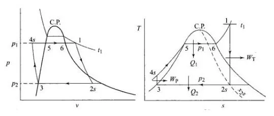
• The efficiency of the Steam Cycle is given by
  `η=((Wn/Q1)=((Wt-Wp)/Q1))
• Applying the Steady Flow Energy Equation (SFEE) to all the process, neglecting the Friction losses and changs in Kinetic & Potential Energy,

1. Q1-h1-h4 @Boiler
2. Wt-h1-h2 @Turbine Q2-h2-h3 @Condenser
3. Wp-h4-h3 @Pump

• The Capacity of the Steam Plant is often expressed interms of Steam Rate (SR) or Specific Steam Consumption (SSC)

S.S.C = ((3600/Wn)(kg/kwh))

Required Inputs:

• Turbine Inlet temperature = 400° C
• Turbine Inlet Pressure = 30 bars
• Turbine Outlet Pressure = 0.05 bars = Condenser Inlet Pressure

Program code :

%Rankine Cycle Simulator

close all
clear all
clc

disp('RANKINE CYCLE SIMULATOR')

disp('1-2 is isentropic expansion in turbine')

disp('2-3 is constant pressure heat rejection in condenser')

disp('3-4 is isentropic compression in pump')

disp('4-1 is constant pressure heat addition in boiler')

p1=input('enter the pressure at the inlet of turbine (in bar) : ');

t1=input('enter the temp at the inlet of turbine (in degree C): ');

p2=input('enter the pressure at the inlet of condenser (in bar): ');

fprintf('rRESULTSrn')

%stage 1 (turbine inlet)
s1= XSteam('s_pT', p1,t1);
h1=XSteam('h_pT', p1,t1);

%stage 2 condenser inlet
sf2 = XSteam('sL_p',p2);
sg2 =XSteam('sV_p',p2);
hf2 = XSteam('hL_p',p2);
hg2= XSteam('hV_p',p2);

s2 = s1;
t2 = XSteam('Tsat_p',p2);

%splitting the formulae
x2=((s2-sf2)/(sg2-sf2));
h2=hf2+(x2*(hg2-hf2));

%stage3 (pump inlet)
p3=p2;
t3=XSteam('Tsat_p', p2);
s3=XSteam('sL_p',p3);
h3=XSteam('hL_p',p3);
cp4= XSteam('cpL_p',p3);
CV4 = XSteam('cvL_p',p3);

gamma =(cp4/CV4);
g = (gamma- 1)/gamma;

%stage 4(boiler inlet)
p4=p1;
s4=s3;
h4 = XSteam('h_ps',p4, s4);
t4=t3*((p4/p3)^g);

%turbine work
wt=h1-h2;

%pump work
wp=h4-h3;

%network
w_net=wt-wp;

%Heat in and out of the system
q_in=h1-h4;
q_out=h2-h3;
q_in=h1-h4;
q_out=h2-h3;

n=w_net/q_in;
np=n*100;

SSC=3600/w_net;
tf_sat=XSteam ('Tsat_p',p1);
sf_sat=XSteam ('sL_p',p1);
hf_sat=XSteam ('hL_p', p1);
sg_sat=XSteam('sV_p',p1);
hg_sat=XSteam('hV_p', p1);

%plot figure 1
figure(1)
hold on
temp=linspace(0, 400, 1000);

for i = 1:length (temp)
aa(i) =XSteam('sL_T', temp(i));

end

for j = 1:length(temp)
bb (j)=XSteam('sV_T', temp(j));

end

plot (aa, temp, 'color', 'b')
plot (bb, temp, 'color', 'b')

temp=(XSteam('Tsat_p', p1));
t0=linspace(temp, t1,300);

for i=1:length(t0)
c11(i)=XSteam('s_pt',p1,t0(i));

end

t5=XSteam('Tsat_p',p4);
s5=XSteam('sL_T', t5);

plot([s1 s2], [t1 t2], 'color', 'r')
plot([s2 s3], [t2 t3], 'color', 'g')
plot([s3 s4], [t3 t4], 'color', 'b')
plot([s4 s5], [t4 t5], 'color', 'c')
plot([sf_sat sg_sat], [tf_sat tf_sat], 'color', 'y')
plot(c11,t0,'color','m')
legend('Saturation Curve L', 'Saturation Curve V', 'Turbine', 'condenser', 'pump', 'boiler', 'location', 'northwest')
title('T-S diagram')
xlabel('entropy(KJ/kgK)')
ylabel('Temperature(K)')

text (s1,t1, '1');
text (s2, t2, '2');
text(s3, t3, '3');
text (s4, t4, '4');
text (s5, t5, '4s');
text(sg_sat, tf_sat, '1s');

%plotting figure 2

figure (2)

hold on

temp1=linspace(0,400, 1000);
for i=1:length(temp1)

cc(i)=XSteam('hL_T', temp1(i));

end

for j=1:length(temp1)
dd (j)=XSteam('hV_T', temp1(j));

end

plot(aa, cc, 'color', 'b')
plot (bb, dd, 'color', 'c')
plot([s1 s2], [h1 h2], 'color', 'r')
plot([s2 s3], [h2 h3], 'color', 'g')
plot([s3 s4], [h3 h4], 'color', 'r')
plot([s4 s1], [h4 h1], 'color', 'g')
legend('Saturation Curve L', 'Saturation Curve V', 'Turbine', 'condenser', 'pump', 'boiler', 'location', 'northwest')
title('H-S diagram')
xlabel('entropy(KJ/KgK)')
ylabel('enthalpy(KJ/Kg)')

text (s1,h1, '1');
text (s2, h2, '2');
text (s3,h3, '3');
text (s4, h4, '4');

%printing the output

fprintf('at stage point 1:n')
fprintf('P1 is : %f barn',p1)
fprintf('T1 is %f deg celsiusn',p1)
fprintf('T1 is :%f KJ/kgn',h1)
fprintf('S1 is: %f KJ/KgKrn', s1)

disp('at state point 2:')
fprintf('P2 is: %f Barn',p2)
fprintf('T2 is: %f deg celsiusn', t2)
fprintf('H2 is: %f KJ/Kgn',h2)
fprintf('S2 is: %f KJ/KgKn', s2)
fprintf('X is : %f rn',x2)

disp('at state point 3:')
fprintf('P3 is %f Barn',p3)
fprintf('T3 is : %f deg celsius400n',t3)
fprintf('H3 is : %f KJ/Kgn',h3)
fprintf('S2 is: %f KJ/KgKbn', s3)

disp('at state point 4:')
fprintf('P4 is : %f Barn',p4)
fprintf('T4 is : %f deg celsiusn', t4)
fprintf('H4 is %f KJ/Kgn', h4)
fprintf('S4 is %f KJ/KgKbn', s4)
fprintf('Wt: %f KJ/Kgn', wt)
fprintf('Wp %f KJ/Kgn', wp)
fprintf('Wnet: %f KJ/Kgn',w_net)
fprintf('SSC %f KJ/KWhbn', SSC)
fprintf('Ntherm %f %%n',n*100)

Explaination of code :

• clc, clear all, close all - to clear command window and remove previous variables.
• fprintf - to print required lines in command window. input to get values of input conditions from user.
• XSteam - custom function to get values from steam table.
• if-else - to calculate dryness fraction s2.
• for - to create points to plot dry saturated liquid and vapour line.
• plot - to plot graph based on input
• text - give name to points in plot.
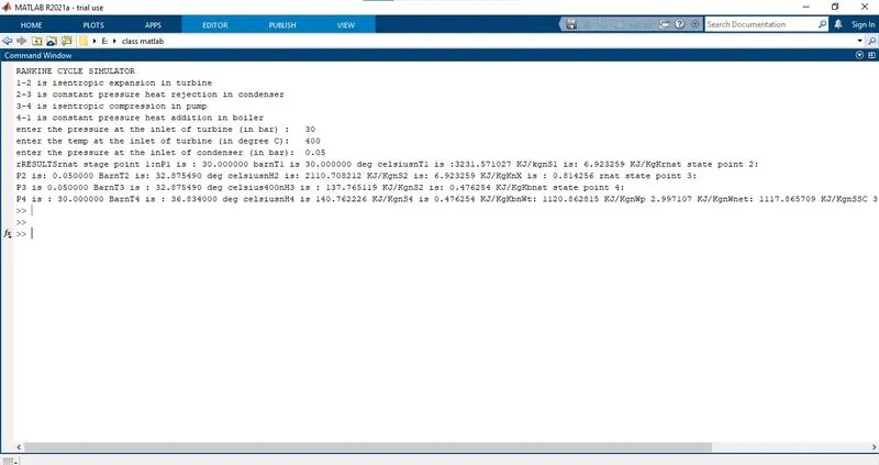
• output -command window will show following output

Results :

T-S DIAGRAM

H-S DIAGRAM

Output of Comment window :

RANKINE CYCLE SIMULATOR

1-2 is isentropic expansion in turbine
2-3 is constant pressure heat rejection in condenser
3-4 is isentropic compression in pump
4-1 is constant pressure heat addition in boiler
enter the pressure at the inlet of turbine (in bar) : 30
enter the temp at the inlet of turbine (in degree C): 400
enter the pressure at the inlet of condenser (in bar): 0.05
rRESULTSrn

at stage point 1:n

P1 is : 30.000000barn

T1 is 30.000000deg celsiusn

T1 is :3231.571027 KJ/kgn

S1 is: 6.923259 KJ/KgKrnat

state point 2:
P2 is: 0.050000 Barn

T2 is: 32.875490deg celsiusn

H2 is: 2110.708212 KJ/Kgn

S2is: 6.923259 KJ/KgK

nX is : 0.814256 rnat state point 3:

P3 is 0.050000 Barn

T3 is : 32.875490 deg celsius400n

H3 is : 137.765119 KJ/Kg

nS2 is: 0.476254 KJ/KgK

bnat state point 4:

P4 is : 30.000000 Barn

T4 is : 36.834000 deg celsiusn

H4 is 140.762226 KJ/Kgn

S4 is 0.476254 KJ/KgK

bnWt: 1120.862815 KJ/Kg

nWp 2.997107 KJ/Kgn

Wnet: 1117.865709 KJ/Kg

nSSC 3.220423 KJ/K

WhbnNtherm 36.167417 %n

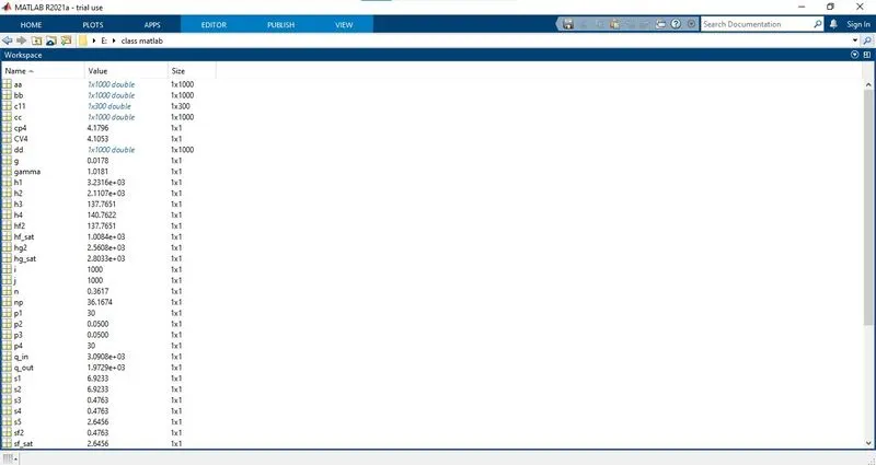
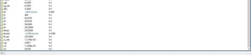
Workspace Output