Project 2 - Rankine cycle Simulator
RANKINE CYCLE
The Rankine cycle is the fundamental operating cycle of all power plants where an operating fluid is continuously evaporated and condensed. The selection of operating fluid depends mainly on the available temperature range. Fig1 shows the idealized Rankine cycle.
The pressure-enthalpy (p-h) and temperature-entropy (T-s) diagrams of this cycle are given in Fig.2. The Rankine cycle operates in the following steps:
-
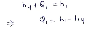
4-1 Isobaric Heat Transfer. High pressure liquid enters the boiler from the feed pump and is heated to the saturation temperature . Further addition of energy causes evaporation of the liquid until it is fully converted to saturated steam.
-
-
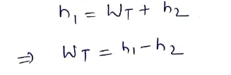
1-2 Isentropic Expansion. The vapor is expanded in the turbine, thus producing work which may be converted to electricity. In practice, the expansion is limited by the temperature of the cooling medium and by the erosion of the turbine blades by liquid entrainment in the vapor stream as the process moves further into the two-phase region. Exit vapor qualities should be greater than 90%.
-
-
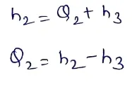
2-3 Isobaric Heat Rejection. The vapor-liquid mixture leaving the turbine (4) is condensed at low pressure, usually in a surface condenser using cooling water. In well designed and maintained condensers, the pressure of the vapor is well below atmospheric pressure, approaching the saturation pressure of the operating fluid at the cooling water temperature.
-
-
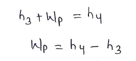
3-4 Isentropic Compression. The pressure of the condensate is raised in the feed pump. Because of the low specific volume of liquids, the pump work is relatively small and often neglected in thermodynamic calculations.
-
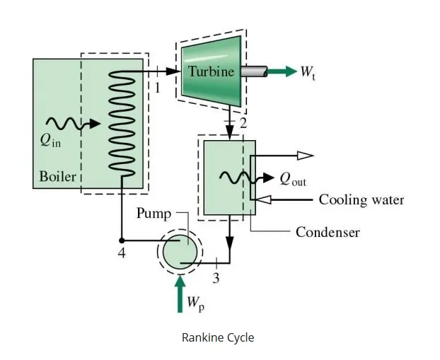
- fig1.
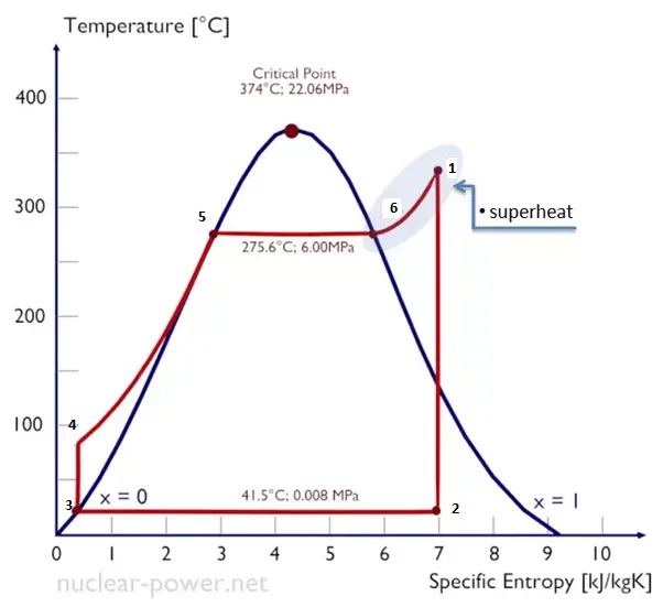
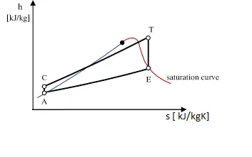
fig. 2
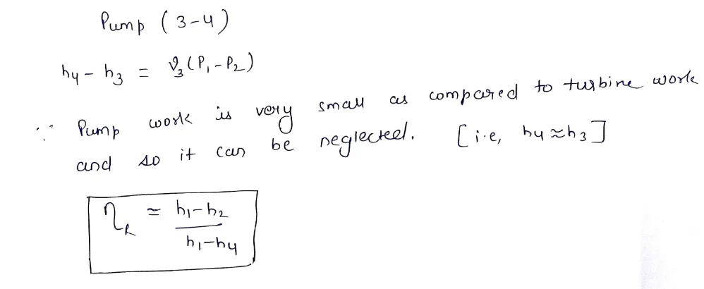
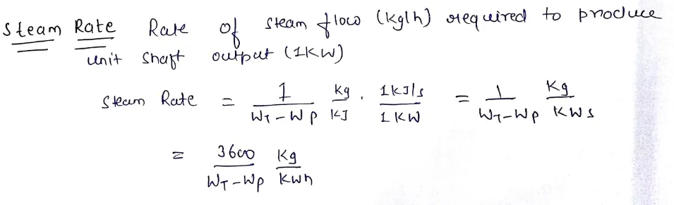
Thermal Efficiency :

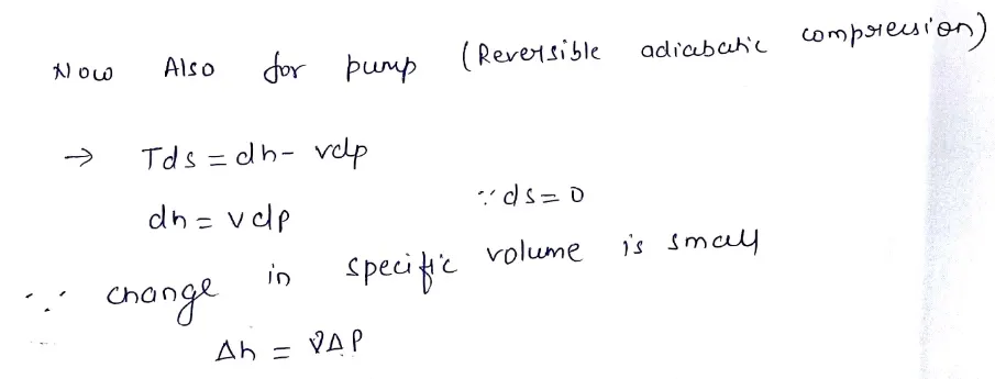
 MAIN CODE
clear all
close all
clc

%process description
fprintf('1-2 Isobaric Heat Addition\n')
fprintf('2-3 Isentropic Expansion\n')
fprintf('3-4 Isobaric Heat Rejection\n')
fprintf('4-1 Isentropic Compression\n')

%initial Inputs to be entered in command window
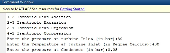
p1 = input('Enter the pressure at turbine Inlet (in bar):');
T1 = input('Enter the Temperature at turbine Inlet (in Degree Celcius):');
p2 = input('Enter the pressure at Condensor (in bar):');

%State points calculation
%Stae point 1
h1 = XSteam('h_pt',p1,T1);
s1 = XSteam('s_pt',p1,T1);

%State point 2
s2=s1;
sf2 = XSteam('sL_p',p2);
sg2 = XSteam('sV_p',p2);
hf2 = XSteam('hL_p',p2);
hg2 = XSteam('hV_p',p2);
x2 = ((s2-sf2)/(sg2-sf2));
h2 = hf2+ x2*(hg2-hf2);
T2 = XSteam('T_hs',h2,s2);

%State point 3
p3 = p2;
s3 = XSteam('sL_p',p3);
h3 = XSteam('hL_p',p3);
T3 = T2;

%State point 4
s4 = s3;
p4 = p1;
Cp4 = XSteam('Cp_ps',p4,s4);
Cv4 = XSteam('Cv_ps',p4,s4);
Y = Cp4/Cv4;
n = (Y-1)/Y;
T4 =  T3*(p4/p3)^n;

%Work done by turbine
Wt = h1-h2;

%Work done to operate pump
v3 = XSteam('vL_p',p3);
Wp = v3*(p4-p3)*100;
h4 = h3 + Wp;

%Net Work
Wnet = Wt - Wp;

%Heat supplied into the System
Qin = h1 - h4;

%Heat Rejected from the system
Qout = h2 - h3;

%Thermal Efficiency
T_eff = (Wnet/Qin)*100;

%Specific Steam Consumption | SSC = mass flow rate/power
SSC = (3600/Wnet);

%Back Work ratio
BW = (Wp/Wt);

%Saurated Liquid and vapor points calculation
T6 = XSteam('Tsat_p',p1);
s5 = XSteam('sL_p',p1);
s6 = XSteam('sV_p',p1);
h5 = XSteam('hL_p',p1);
h6 = XSteam('hV_p',p1);
T5 = T6;

%Printing results
fprintf('\nResults\n');
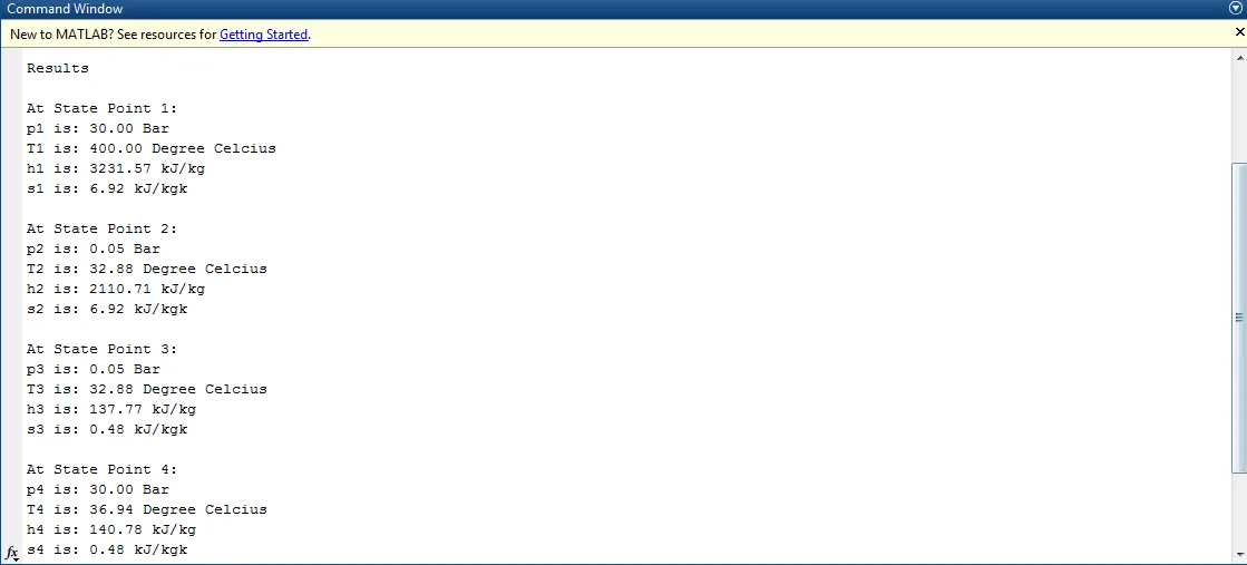
fprintf('\nAt State Point 1:\np1 is: %4.2f Bar\nT1 is: %4.2f Degree Celcius\nh1 is: %4.2f kJ/kg\ns1 is: %4.2f kJ/kgk\n\n',p1,T1,h1,s1);
fprintf('At State Point 2:\np2 is: %4.2f Bar\nT2 is: %4.2f Degree Celcius\nh2 is: %4.2f kJ/kg\ns2 is: %4.2f kJ/kgk\n\n',p2,T2,h2,s2);
fprintf('At State Point 3:\np3 is: %4.2f Bar\nT3 is: %4.2f Degree Celcius\nh3 is: %4.2f kJ/kg\ns3 is: %4.2f kJ/kgk\n\n',p3,T3,h3,s3);
fprintf('At State Point 4:\np4 is: %4.2f Bar\nT4 is: %4.2f Degree Celcius\nh4 is: %4.2f kJ/kg\ns4 is: %4.2f kJ/kgk\n\n',p4,T4,h4,s4);
fprintf('Wt is: %4.2f kJ/kg\nWp is: %4.2f kJ/kg\nWnet is: %4.2f kJ/kg\nThermalEfficiency is: %4.2f percent\nSSC is: %4.2fkg/kWh',Wt,Wp,Wnet,T_eff,SSC);

%plotting Saturation curve and T-S diagram
T = linspace(1,375,1000);
for i = 1:length(T);
    sf(i) = XSteam('sL_T',T(i));
    sg(i) = XSteam('sV_T',T(i));
    hf(i) = XSteam('hL_T',T(i));
    hg(i) = XSteam('hV_T',T(i));
end

figure(1)
hold on
plot(sf,T,'color','r','linewidth',1.5)
plot(sg,T,'color','r','linewidth',1.5)

plot([s1 s2],[T1 T2],[s2 s3],[T2 T3],[s3 s4],[T3 T4],[s4 s5],[T4 T5],[s5 s6],[T5 T6],[s6 s1],[T6 T1],'marker','o','markersize',5,'color','k','linewidth',2);
text(s1+0.2,T1,'1')
text(s2+0.2,T2,'2')
text(s3+0.2,T3-4,'3')
text(s4-0.3,T4+4,'4')
text(s5-0.4,T5+5,'5')
text(s6+0.2,T6,'6')
xlabel('Entropy (kJ/kgK)')
ylabel('Temperatur (K)')
legend('saturation curve')

figure(2)
hold on
plot(sg,hg,'color','r','linewidth',1.5)
plot(sf,hf,'color','r','linewidth',1.5)

plot([s1 s2],[h1 h2],[s2 s3],[h2 h3],[s3 s4],[h3 h4],[s4 s1],[h4 h1],'marker','o','markersize',3,'color','k','linewidth',2);
text(s1+0.1,h1,'1')
text(s2+0.1,h2,'2')
text(s3+0.2,h3-4,'3')
text(s4-0.3,h4+4,'4')
xlabel('Entropy (kJ/kgK)')
ylabel('Enthalpy (kJ/K)')
legend('saturation curve')
EXPLANATION
- First Command Window and Workspace are being cleared and closed.
- Rankine Cycle Process description is mentioned using pfrintf command.
- Initial inputs were given using input command and they will be given in the command window once the code is executed.
- Stae points variables such as Enthalpy, Entropy were extracted from XSteam file as a function of Temperature and Pressure, for eg. s1 = XSteam('s_pt',p1,T1); , this gives us the Entropy of water at given pressure and temperature.
- Thermodynamic relations were used to further calculate all the State point variables and extract their data from XSteam
- Enthaply and Entropy at Saturated liquid and vapor state points are also calculated using XSteam library
- Followed by calculation of Work done by the Turbine (Wt) and work done on the Pump (Wp) and the Net Work done.
- Heat supplied into the system and Heat Rejected from the System is also calculated.
- After that, Thermal Efficiency is calculated which nothing but (Net Work done/Heat supplied )
- It follows by the Calculation of Specific Steam Consumption and Back Work ratio.
- After Calculation of all the State variables and Important parameters and results, these results are printed in the command window using fprintf command.
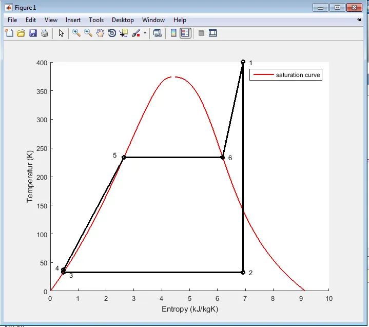
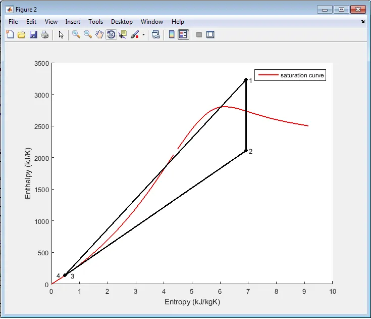
- This is finally followed by plotting of T-s and h-s diagram using plot command and using the calculations of state point variables prior to this.
RESULTS
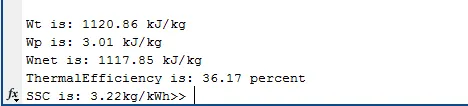
PLOTS
1. T-s DIAGRAM
2. h-s Diagram
Errors and Rectification
1.
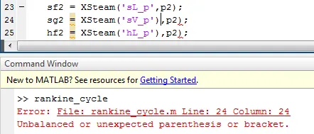
This is a syntax error as we can see in line 24 and 25 we have an extra bracket after sV_p and hL_p respectively. This error was resolved just by removing those brackets.
REFERENCES
- http://www.thermopedia.com/content/1072/
- https://medium.com/@ashwinpalo/how-to-calculate-thermal-efficiency-of-rankine-cycle-37a7dbcadc12
- https://www.nuclear-power.net/nuclear-engineering/thermodynamics/thermodynamic-cycles/rankine-cycle-steam-turbine-cycle/theory-of-rankine-cycle-equations-and-calculation/
- https://medium.com/@ashwinpalo/how-to-calculate-thermal-efficiency-of-rankine-cycle-37a7dbcadc12