Project 2 - Rankine cycle Simulator

RANKINE CYCLE SIMULATION USING MATLAB

OBJECTIVE :

The final objective of this project is to understand the concept of rankine cycle and to devolop a basic program, to calculate state points of rankine cycle . and to add thermodynamic relation to get the points in between the state variables. To plot rankine cycle on T-S and H-S curve

THEORY :

Thermodynamic cycles can be divided into two general categories: power cycles, which produce a net power output, and refrigeration and heat pump cycles, which consume a net power input. The thermodynamic power cycles can be categorized as gas cycles and vapor cycles. In gas cycles, the working fluid remains in the gas phase throughout the entire cycle. In vapor cycles, the working fluid exits as vapor phase during one part of the cycle and as liquid phase during another part of the cycle.

Steam power plants run vapor power cycles with water as the working fluid. This section introduces the ideal cycle for vapor power cycle - Rankine cycle.

RANKINE CYCLE THE IDEAL CYCLE FOR VAPOUR POWER CYCLE :

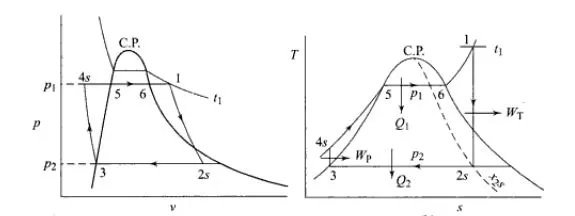
The Rankine cycle is an ideal cycle if water passes through the four components without irreversibilities and pressure drops. The ideal Rankine cycle consists of the following four processes, as shown on the T-s diagram :

• 1-2: Isentropic compression in a pump
• 2-3: Constant pressure heat addition in a boiler
• 3-4: Isentropic expansion in a turbine
• 4-1: Constant pressure heat rejection in a condenser

Vapor power plants generate electrical power by using fuels like coal, oil or natural gas. The schematic of a vapor power plant is shown on the left. The entire power plant can be broken down into four major subsystems.

• Subsystem A: Energy conversion from heat to work
• Subsystem B: Energy source and waste removal required to vaporize the water
• Subsystem C: Electric generator
• Subsystem D: Cooling water system

The thermodynamic cycle in subsystem A is called the Rankine cycle. Subsystem A consists of a boiler, turbine, condenser and a pump. Fuel, burned in the boiler, heats the water to generate superheated steam (subsystem B). This steam is used to run the turbine which powers the generator. Electrical energy is generated when the generator windings rotate in a strong magnetic field (subsystem C). After the steam leaves the turbine, it is cooled to its liquid state in the condenser by transferring heat to the cooling water system (subsystem D). The liquid is pressurized by the pump prior to going back to the boiler.

All four components associated with the ideal Rankine cycle are steady-flow devices, and thus all four processes that make up the Rankine cycle can be analyzed as steady-flow process. The kinetic and potential energy changes of water are small relative to the heat and work terms, are thus neglected. Energy analysis of the four components are given below.

Pump (process 1-2): Pump pressurized the liquid water from the condenser prior to going back to the boiler. Assuming no heat transfer with the surroundings, the ENERGY BALENCE IN THE PUMP is

w_{pump, in} = h₂ - h₁

Boiler (process 2-3): Liquid water enters the boiler and is heated to superheated state in the boiler. The energy balance in the boiler is

q_in = h₃ - h₂

Turbine (process 3-4): Steam from the boiler, which has an elevated temperature and pressure, expands through the turbine to produce work and then is discharged to the condenser with relatively low pressure. Neglecting heat transfer with the surroundings, the ENERGY BALENCE IN THE TURBINE is

w_{turbine, out} = h₃ - h₄

Condenser (process 4-1): Steam from the turbine is condensed to liquid water in the condenser. The energy balance in the condenser is

q_out = h₄ - h₁

For the whole cycle, the energy balance can be obtained by summarizing the four energy equations above. It yields,

(q_in- q_out) - (w_{turbine, out} - w_{pump, in}) = 0

The thermal efficiency of the Rankine cycle is determined from

η_th = w_{net ,out}/q_in = 1 - q_out/q_in

where the net work output from the cycle is

w_{net ,out} = w_{turbine, out} - w_{pump, in}

MATLAB CODE :

close all
clear all
clc
% Print Process Description
fprintf('1-2 Isobaric heat Transfern')
fprintf('2-3 Isentropic Expansionn')
fprintf('3-4 Isobaric heat Rejectionn')
fprintf('4-1 Isentropic Compressionn')
%step 1:Enter Inputs
p1 = input('Enter the Pressure at the Turbine Inlet (in bar):');
T1 = input('Enter the Temperature at the Turbineinlet (in Degree Celcius):');
p2 = input('Enter the Pressure at the Condensor (in bar):');
%step 2: Calculate each state point values.
% state point 1
h1 = XSteam('h_pt',p1,T1);
s1 = XSteam('s_pt',p1,T1);
%step 3: state point 2
s2=s1;
sf2 = XSteam('sL_p',p2);
sg2 = XSteam('sV_p',p2);
hf2 = XSteam('hL_p',p2);
hg2 = XSteam('hV_p',p2); %x2 = (s2-sf2)/(sg2-sf2);
s2 = sg2;
h2 = hg2; %hf2 +(x2*(hg2-hf2));
T2=XSteam('T_hs',h2,s2);
%step 4: state point 3T3=T2;
p3= p2;
s3=XSteam('sL_T',T3);
h3=XSteam('hL_T',T3);
v3 = XSteam('vL_p',p2);
%step 5: state point 4
p4 =p1;
s4= s3;
Cp4 = XSteam('Cp_ps',p4,s4);
Cv4 = XSteam('Cv_ps',p4,s4);
gamma = Cp4/Cv4;
r = (gamma - 1)/gamma;
T4 = T3 *(p4/p3)^r;
%step 6: Calculate other output values.
Wt = h1-h2; % Turbine Work 
Wp = v3*(p1-p2)*100; % Pump Work
h4 = Wp + h3;
W_net = Wt-Wp; 
% Net Work unit in kj/kg
Qs = h1 - h4;%heat suppied
N_per = (W_net/Qs)*100;%Efficiency
steam_rate = 3600/(Wt - Wp);%Steam rate per second
%step 7: state point 5 and 6 which help in plotting
T5=XSteam('Tsat_p',p1);
T6=T5;s5=XSteam('sL_p',p1);
s6=XSteam('sV_p',p1);
h5=XSteam('hL_p',p1);
h6=XSteam('hV_p',p1);
%step 8: print all state poont values to show.
fprintf('n------------------RESULT------------------n')
fprintf('At State point 1:nP1 is : %4.2f BarnT1 is : %4.2f Degree CelciusnH1 is : %4.2f kJ/kgnS1 is : %4.2f kJ/kgknn',p1,T1,h1,s1)
fprintf('At State point 2:nP2 is : %4.2f BarnT2 is : %4.2f Degree CelciusnH2 is : %4.2f kJ/kgnS2 is : %4.2f kJ/kgknn',p2,T2,h2,s2)
fprintf('At State point 3:nP3 is : %4.2f BarnT3 is : %4.2f Degree CelciusnH3 is : %4.2f kJ/kgnS3 is : %4.2f kJ/kgknn',p3,T3,h3,s3)
fprintf('At State point 4:nP4 is : %4.2f BarnT4 is : %4.2f Degree CelciusnH4 is : %4.2f kJ/kgnS4 is : %4.2f kJ/kgknn',p4,T4,h4,s4)
fprintf('Wt is :%4.2f kJ/kgnWp is : %4.2f kJ/kgnWnet is : %4.2f kJ/kgnNtherm is : %4.2f percentnS.S.C is : %4.2f kg/kWh',Wt,Wp,W_net,N_per,steam_rate)
%step 9:plot T-S Diagram
subplot(1,2,1)
T_rankine = linspace(T5,T1,5000);
for i = 1:length(T_rankine) 
    s_rankine(i) = XSteam('s_pT',p1,T_rankine(i));
end
plot([s1 s2 s3 s4 s5 s6 s_rankine],[T1 T2 T3 T4 T5 T6 T_rankine],'linewidth',1.5);
hold on
T_curve = linspace(1,400,500);
for i=1:length(T_curve) 
    s_l(i) = XSteam('sL_T',T_curve(i)); 
    s_v(i) = XSteam('sV_T',T_curve(i));
    h_l(i) = XSteam('hL_T',T_curve(i)); 
    h_v(i) = XSteam('hV_T',T_curve(i));
end
plot(s_l,T_curve);
plot(s_v,T_curve);
text(s1,T1,'1','FontSize',15)
text(s2,T2,'2','FontSize',15)
text(s3,T3,'3','FontSize',15,'HorizontalAlignment','right','VerticalAlignment','top')
text(s4,T4,'4','FontSize',15,'HorizontalAlignment','right','VerticalAlignment','bottom')
text(s5,T5,'5','FontSize',15)
text(s6,T6,'6','FontSize',15)
xlabel('Entropy in kJ/KgK');
ylabel('Temperature in Degree Celcius');
%step 10:plot H-S diagram
subplot(1,2,2)
plot([s1 s2 s3 s4 s1],[h1 h2 h3 h4 h1],'linewidth',2)
hold on
plot(s_v,h_v,'color','r')
plot(s_l,h_l,'color','r')
text(s1,h1,'1','FontSize',15)
text(s2,h2,'2','FontSize',15)
text(s3,h3,'3','FontSize',15,'HorizontalAlignment','right','VerticalAlignment','top')
text(s4,h4,'4','FontSize',15,'HorizontalAlignment','right','VerticalAlignment','bottom')
xlabel('Entropy in kJ/KgK')
ylabel('Enthalpy in kJ/kg')

Explanation of code :

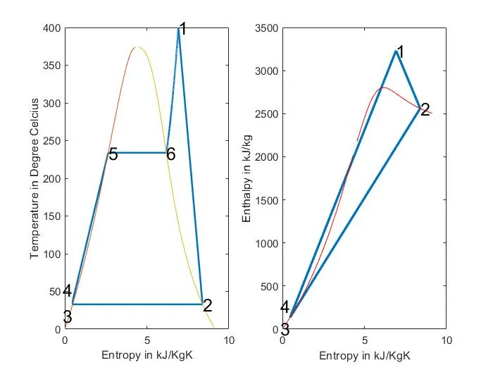
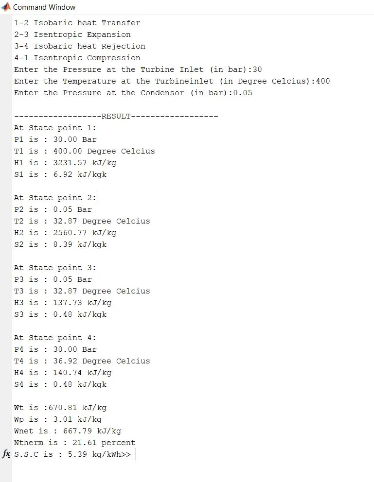
The Program begins with clear all, close all, clc to erase the workspace and plots..Input variables p1,T1,p2 are given by input command whose values are entered in command window while executing the Program.@State-1, Values for Enthalpy & Entropy are extracted as a function of Pressure & Temperature.h_pT, s_pT, hL_p, sV_p etc.... are the default variables whose value is stored in XSteam file.Similarly, all the variables for all states are extracted using a suitable format.[**The Formulae for the State Variables and other depending factors are referred from Power Plant Reference Books.]Pressure, Temperature, Enthalpy, Entropy for all the State Variables are Extracted as a function of the dependent variable from the XSteam File.@State 2 is a Condenser inlet where the High-Pressure Steam is converted into Low-Pressure Water and hence Dryness Fraction, Enthalpy & Entropy for Saturated Vapour & Saturated Water are considered to Calculate the Specific Enthalpy.@State-3 The water is condensed back to its Saturation Temperature and fed to the Pump, This temperature of water at the exit of the Condenser and entry of Pump is the same.@State-4 This is Constant Pressure Heat addition, hence pressure is equal to p1, but the temperature increases on heating at Constant Pressure & Constant Volume as our Entropy remains same and hence Cp/Cv=gamma is considered to find temperature T4.define two more points 5 and 6 to plot cycle in detail.Finally Work done and Heat Evolved & SSC are calculated by basic formulae.To plot the Saturation Curve, a Temperature range is defined using linspace command and for the overall length of this Temperature values of Enthalpy and Entropy are calculated at every temperature point. The Break in the Saturation Curve separates the Liquid Phase & Vapour Phase.Now all the necessary data is found out, Plotting is done for both T-S & H-S curves using the plot commands. Annotations are assigned using text command.Results of the Cycle Simulation is displayed over Comand window using fprintf command.

RESULT :