Project 2 - Rankine cycle Simulator

IDEAL RANKINE CYCLE SIMULATOR

AIM :

The program in matlab to simulate Rankine Cycle.

PROCEDURE :

The Rankine cycle is an ideal cycle if water passes through the four components without irreversibilities and pressure drops. The ideal Rankine cycle consists of the following four processes, as shown on the T-s diagram

• 1-2: Isentropic expansion in a turbine.
• 2-3: Constant pressure heat rejection in a condenser.
• 3-4: Isentropic compression in a pump.
• 4-1: Constant pressure heat addition in a boiler.

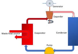
All four components associated with the ideal Rankine cycle are steady-flow devices, and thus all four processes that make up the Rankine cycle can be analyzed as steady-flow process. The kinetic and potential energy changes of water are small relative to the heat and work terms, are thus neglected. Energy analysis of the four components are given below.

(process 1-2): Pump pressurized the liquid water from the condenser prior to going back to the boiler. Assuming no heat transfer with the surroundings, the energy balance in the pump is,

w_{pump, in} = h₂ - h₁

(process 2-3): Liquid water enters the boiler and is heated to superheated state in the boiler. The energy balance in the boiler is,

q_in = h₃ - h₂

(process 3-4): Steam from the boiler, which has an elevated temperature and pressure, expands through the turbine to produce work and then is discharged to the condenser with relatively low pressure. Neglecting heat transfer with the surroundings, the energy balance in the turbine is

w_{turbine, out} = h₃ - h₄

(process 4-1): Steam from the turbine is condensed to liquid water in the condenser. The energy balance in the condenser is

q_out = h₄ - h₁

Program for Rankine cycle,

XSteam Table link : https://drive.google.com/open?id=1RK_fvrOj38CIaQvmLT1S3daqHnxKCGU-

clear all
close all
clc

% RANKINE_CYCLE_SIMULATOR
fprintf('RANKINE CYCLE SIMULATOR\n')
fprintf('1-2 isentropic reversible adiabatic expansion\n')
fprintf('2-3 constant pressure heat rejection in the condenser \n')
fprintf('3-4 isentropic pressure to the boiler\n')
fprintf('4-1 heat supplied at constant pressure by boiler\n')

% inputs
p1 = 30;
t1 = 400;
p2 = 5;


% % calculation
%h_pT	Entalpy as a function of pressure and temperature.
h1 = XSteam('h_pT',p1,t1);
%s_pT	Specific entropy as a function of pressure and temperature
s1 = XSteam('s_pT',p1,t1);
%vV_p	Saturated vapour volume
v1 = XSteam('vV_p',p1);

% input
s2 = s1;

%Tsat_p	Saturation temperature
t2 = XSteam('Tsat_p',p2);
%vV_p	Saturated vapour volume
v2 = XSteam('vV_p',p2);


% % h2=hf2+x2*(hg2-hf2) | x2=(s2-sf2)/(sg2-sf2)
%sL_p	Saturated liquid entropy
sf2 = XSteam('sL_p',p2);
%sV_p	Saturated vapour entropy
sg2 = XSteam('sV_p',p2);
%hL_p	Saturated liquid enthalpy
hf2 = XSteam('hL_p',p2);
%hV_p	Saturated vapour enthalpy
hg2 = XSteam('hV_p',p2);

x2 = (s2-sf2)/(sg2-sf2);

h2=hf2+x2*(hg2-hf2);

% inputs
p3 = p2;
t3 =t2;
%sL_p	Saturated liquid entropy
s3 = XSteam('sL_p',p3);
%hL_p	Saturated liquid enthalpy
h3 = XSteam('hL_p',p3);
%vL_p	Saturated liquid volume
v3 = XSteam('vL_p',p3);

% inputs
s4 = s3;
p4 = p1;

% % t4 = t3*(p4/p3)^k | k=(gamma-1)/gamma | gamma= cp4/cv4
%Cp_ps	Specific isobaric heat capacity as a function of pressure and entropy
cp4 = XSteam('Cp_ps',p4,s4);
%Cv_ps	Specific isochoric heat capacity as a function of pressure and entropy
cv4 = XSteam('Cv_ps',p4,s4);

gamma = cp4/cv4;

k = (gamma-1)/gamma;

t4 = t3*(p4/p3)^k;


% total work output(w_net) = w_turbine - w_pump
w_turbine = h1-h2;
% w_pump = h4-h3 = v3(p4-p3)
w_pump = v3*(p4-p3);
w_net = w_turbine - w_pump;

h4 = h3 + w_pump;

%vL_p	Saturated liquid volume
v4 = XSteam('vL_p',p4);


% inputs
p5 = p1;

%Tsat_p	Saturation temperature
t5 = XSteam('Tsat_p',p5);
%hL_p	Saturated liquid enthalpy
h5 = XSteam('hL_p',p5);
%sL_p	Saturated liquid entropy
s5 = XSteam('sL_p',p5);

% inputs
p6 = p5;

%Tsat_p	Saturation temperature
t6 = XSteam('Tsat_p',p6);
%hL_p	Saturated liquid enthalpy
h6 = XSteam('hL_p',p6);
%sL_p	Saturated liquid entropy
s6 = XSteam('sL_p',p6);

T = linspace(1,t1,400);
for i = 1:length(T)
    Hl(i) = XSteam('hL_T',T(i));
    Hv(i) = XSteam('hV_T',T(i));
    Sl(i) = XSteam('sL_T',T(i));
    Sv(i) = XSteam('sV_T',T(i));
end

% plots

subplot(1,2,1)
plot([s1 s2 s3 s4 s5 s6 s1],[t1 t2 t3 t4 t5 t6 t1])
hold on
plot(Sl,T,'color','r')
plot(Sv,T,'color','r')
axis([0 10 0 600])
xlabel('Entropy')
ylabel('Temperature')
title('T-S Diagram')
text(s1,t1,'1')
text(s2,t2,'2')
text(s3,t3,'3')
text(s4,t4,'4')
text(s5,t5,'5')


subplot(1,2,2)
plot([s1 s2 s3 s4 s5 s6 s1],[h1 h2 h3 h4 h5 h6 h1])
hold on
plot(Sl,Hl,'color','r')
plot(Sv,Hv,'color','r')
xlabel('Entropy')
ylabel('Enthalpy')
title('H-S Diagram')
text(s1,h1,'1')
text(s2,h2,'2')
text(s3,h3,'3')
text(s4,h4,'4','horizontalalignment','right')
text(s5,h5,'5')

% % outputs result
fprintf('\n inputs \n')
fprintf('Enter the pressure at turbine inlet(in bar): %.2f\n',p1)
fprintf('Enter the temperature at turbine inlet(in degree celcius): %.2f\n',t1)
fprintf('Enter the pressure at the condenser(in bar): %.2f\n',p2)

fprintf('\nstate 1\n')
fprintf('p1 = %.3f (bar)\n',p1)
fprintf('t1 = %.3f (celsius)\n',t1)
fprintf('h1 = %.3f (kj/kg)\n',h1)
fprintf('s1 = %.3f (kj/kg*k)\n',s1)
fprintf('v1 = %.3f (m^3)\n',v1)

fprintf('\nstate 2\n')
fprintf('p2 = %.3f (bar)\n',p2)
fprintf('t2 = %.3f (celsius)\n',t2)
fprintf('h2 = %.3f (kj/kg)\n',h2)
fprintf('s2 = %.3f (kj/kg*k)\n',s2)
fprintf('v2 = %.3f (m^3)\n',v2)

fprintf('\nstate 3\n')
fprintf('p3 = %.3f (bar)\n',p3)
fprintf('t3 = %.3f (celsius)\n',t3)
fprintf('h3 = %.3f (kj/kg)\n',h3)
fprintf('s3 = %.3f (kj/kg*k)\n',s3)
fprintf('v3 = %.3f (m^3)\n',v3)

fprintf('\nstate 4\n')
fprintf('p4 = %.3f (bar)\n',p4)
fprintf('t4 = %.3f (celsius)\n',t4)
fprintf('h4 = %.3f (kj/kg)\n',h4)
fprintf('s4 = %.3f (kj/kg*k)\n',s4)
fprintf('v4 = %.3f (m^3)\n',v4)

fprintf('\nwork_Turbine = %.3f (kj/kg)\n',w_turbine)
fprintf('work_Pump = %.3f (kj/kg)\n',w_pump)
fprintf('work_Net = %.3f (kj/kg)\n',w_net)

As per the given inputs and XSteam we are calculating enthalpy , entropy , pressure , volume & temperature for all four process. And the output which is plotted by using plot command. Also the process which is written in the graph by using text command. To execute the result in the command window we are using fprintf command.

RESULTS :

Outputs,

CONCLUSION :

Thus the program in matlab to simulate Rankine Cycle is concluded sucessfully