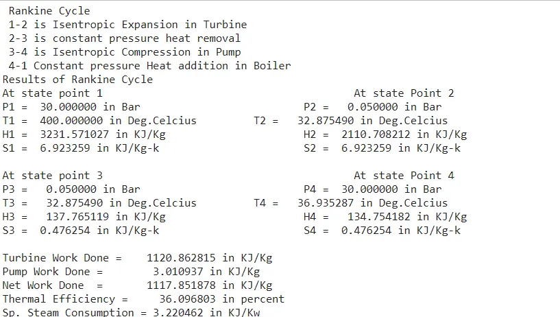
The Rankine Cycle is a fundamental thermodynamic cycle that is widely utilized in power generation systems, particularly in steam power plants. Named after William John Macquorn Rankine, this cycle describes the conversion of heat into mechanical work through the use of a working fluid, typically water or steam. The Rankine Cycle consists of four main processes: isentropic expansion, constant pressure heat removal, isentropic compression, and constant pressure heat addition. These processes occur in devices such as turbines, condensers, pumps, and boilers.
The XSteam library is a valuable tool in thermodynamic analysis, providing a set of functions for steam and water properties based on the International Association for the Properties of Water and Steam (IAPWS) formulations. This library allows engineers and researchers to access essential steam property data, such as enthalpy, entropy, temperature, and pressure, facilitating the design and analysis of energy systems, including those based on the Rankine Cycle.
The XSteam library offers functions for obtaining steam properties, including 'h_pT' for enthalpy at specified pressure and temperature, 's_pT' for entropy, 'vL_p' for saturated liquid volume, and many more.
clear all
close all
clc
% Rankine Cycle Simulator
fprintf(' Rankine Cycle\n ')
fprintf('1-2 is Isentropic Expansion in Turbine\n')
fprintf(' 2-3 is constant pressure heat removal\n')
fprintf(' 3-4 is Isentropic Compression in Pump \n')
fprintf(' 4-1 Constant pressure Heat addition in Boiler\n')
% Entering the input data for calculation of state points
p1 = 30; %Pressure at Turbine Inlet
T1 = 400; %Temperature at Turbine Inlet
p2 = 0.05; %Pressure at Condenser
% Taking data from Xsteam file for State point 1
h1 = XSteam('h_pT', p1, T1); % Enthaply at pressure and Temp 1
s1 = XSteam('s_pT', p1, T1); % Entropy at pressure and Temp 1
% Taking data from Xsteam file for State point 2
s2 = s1; % Because of Isentropic Expansion
sf2 = XSteam('sL_p', p2); % Saturated liquid entropy at pressure 2
sg2 = XSteam('sV_p', p2); % Saturated vapour entropy at pressure 2
x2 = (s2-sf2)/(sg2-sf2); % Vapour Fraction at state point 2
hf2 = XSteam('hL_p', p2); % Saturated liquid Enthalpy at pressure 2
hg2 = XSteam('hV_p', p2); % Saturated vapour Enthalpy at pressure 2
h2 = hf2 + (x2*(hg2-hf2)); % Enthalpy at state point 2
% Taking data from Xsteam file for state point 3
p3 = p2; % Constant Pressure heat removal process
s3 = XSteam('sL_p', p3); % Saturated liquid entropy at Pressure 3
h3 = XSteam('hL_p', p3); % Saturated liquid Enthalpy at Pressure 3
% Taking data from Xsteam file for State point 4
s4 = s3; % Isentropic Compression process
p4 = p1; % Constant Pressure heat rejection
% Work done in Turbine for the rankine cycle
W_T = h1-h2;
% Work done required for pump
v3 = XSteam('vL_p',p3); % Saturated Liquid Vapour at pressure 3
W_P = v3*(p4-p3)*100; % Work done for pump
h4 = h3 - W_P; % Enthalpy at State point 4
% Net work done for Rankine Cycle
W_net = W_T - W_P;
% Heat Addition to System
Q_in = h1-h4;
% Heat Rejection from System
Q_out = h2-h3;
% Thermal Efficiency of Rankine Cycle
T_eff = (W_net/Q_in)*100;
%specific steam consumption = (Mass flow rate / Net work done)
Sp_S = (3600/W_net);
% Calculation of Temperature at All state Point 2, 3 and 4
T3 = XSteam('Tsat_p',p3); % Saturation Temperature at Pressure 3
T2 = T3; % Becuase of Constant Pressure Heat addition
Cp4 = XSteam('Cp_ps',p4,s4); % Specific isobaric heat capacity
Cv4 = XSteam('Cv_ps',p4,s4); % Specific isochoric heat capacity
k = Cp4/Cv4;
T4 = T3/((p3/p4)^((k-1)/k)); % Temperature at State point 4
% Calculation of Other constant for saturated liquid and Vapour
T6 = XSteam('Tsat_p', p1); % Saturated Temperature at Pressure 1
s5 = XSteam('sL_p', p1); % Saturated Liquid entropy at pressure 1
s6 = XSteam('sV_p', p1); % Saturated Vapour entropy at Pressure 1
h5 = XSteam('hL_p', p1); % Saturated Liquid Enthalpy at Pressure 1
h6 = XSteam('hV_p', p1); % Saturated Vapour Enthalpy at pressure 1
T5 = T6;
%Plotting for Saturation Line
T = linspace(1,560,1000);
for i = 1:length(T)
sf(i) = XSteam('sL_T' ,T(i)); % Saturated Liquid Entropy
sg(i) = XSteam('sV_T' ,T(i)); % Saturated Vapour Entropy
hf(i) = XSteam('hL_T' ,T(i)); % Saturated Liquid Enthalpy
hg(i) = XSteam('hV_T' ,T(i)); % Saturated Vapour Enthalpy
end
% Plotting T-S Diagram for Rankine Cycle
figure(1)
hold on
plot(sf,T,'color','b','linewidth',2)
plot(sg,T,'color','b','linewidth',2)
plot([s1 s2],[T1 T2], 'color', 'r', 'linewidth',3)
plot([s2 s3],[T2 T3], 'color', 'r', 'linewidth',3)
plot([s3 s4],[T3 T4], 'color', 'r', 'linewidth',3)
plot([s4 s5],[T4 T5], 'color', 'r', 'linewidth',3)
plot([s5 s6],[T5 T6], 'color', 'r', 'linewidth',3)
s_1 = linspace(s6,s1,1000);
for j = 1:length(s_1)
Tc(j) = XSteam('T_ps',p1,s_1(j));
end
plot(s_1,Tc,'color','r','linewidth',3)
text(s1+0.1, T1, '1')
text(s2+0.1, T2, '2')
text(s3, T3-20, '3')
text(s4, T4+20, '4')
title('Temperature Vs Entropy')
xlabel('Entropy (Kj/kg-k)')
ylabel('Temeperature (Deg. Celcius)')
legend('Saturation Curve')
% Plotting H-S Diagram for Rankine Cycle
figure(2)
hold on
plot(sf,hf,'color','b','linewidth',2)
plot(sg,hg,'color','b','linewidth',2)
plot([s1 s2],[h1 h2],'color','r','linewidth',3)
plot([s2 s3],[h2 h3],'color','r','linewidth',3)
plot([s3 s4],[h3 h4],'color','r','linewidth',3)
hc = linspace(h4,h5,100);
for k = 1:length(hc)
s_c(k) = XSteam('s_ph',p1,hc(k));
end
plot(s_c,hc,'color','r','linewidth',3)
plot([s5 s6],[h5 h6],'color','r','linewidth',3)
for l = 1:length(s_1)
h_c(l) = XSteam('h_ps',p1,s_1(l));
end
plot(s_1,h_c,'color','r','linewidth',3)
text(s1+0.1,h1,'1')
text(s2+0.1,h2,'2')
text(s3,h3-100,'3')
text(s4,h4+200,'4')
title('Enthalpy Vs Entropy')
xlabel('Entropy (Kj/kg-k)')
ylabel('Enthalpy (KJ/Kg)')
legend('Saturation Curve')
% Displaying Results in Command window
disp('Results of Rankine Cycle')
fprintf('At state point 1\t\t\t\t\t')
fprintf('At state Point 2\n')
fprintf('P1 = %10f in Bar\t\t\t\t',p1);
fprintf('P2 = %10f in Bar\n',p2);
fprintf('T1 = %11f in Deg.Celcius\t\t',T1);
fprintf('T2 = %11f in Deg.Celcius\n',T2);
fprintf('H1 = %12f in KJ/Kg\t\t\t',h1);
fprintf('H2 = %12f in KJ/Kg\n',h2);
fprintf('S1 = %9f in KJ/Kg-k\t\t\t',s1);
fprintf('S2 = %9f in KJ/Kg-k\n',s2);
fprintf('\n')
fprintf('At state point 3\t\t\t\t\t')
fprintf('At state Point 4\n')
fprintf('P3 = %10f in Bar\t\t\t\t',p3);
fprintf('P4 = %10f in Bar\n',p4);
fprintf('T3 = %11f in Deg.Celcius\t\t',T3);
fprintf('T4 = %11f in Deg.Celcius\n',T4);
fprintf('H3 = %12f in KJ/Kg\t\t\t',h3);
fprintf('H4 = %12f in KJ/Kg\n',h4);
fprintf('S3 = %9f in KJ/Kg-k\t\t\t',s3);
fprintf('S4 = %9f in KJ/Kg-k\n',s4);
fprintf('\n')
fprintf('Turbine Work Done = %14f in KJ/Kg\n',W_T)
fprintf('Pump Work Done = %15f in KJ/Kg\n',W_P)
fprintf('Net Work Done = %17f in KJ/Kg\n',W_net)
fprintf('Thermal Efficiency = %13f in percent\n',T_eff)
fprintf('Sp. Steam Consumption = %f in KJ/Kw\n',Sp_S)
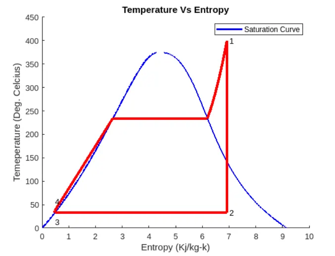
T-S (Temperature vs. Entropy) Diagram: Saturation Curve: The blue curve represents the saturation curve, indicating the boundary between the liquid and vapor phases of water. The curve separates the region of saturated liquid (subcooled) and saturated vapor (superheated). Process Lines (1-2, 2-3, 3-4, 4-5, 5-1): The red lines represent the processes in the Rankine Cycle. Process 1-2: Isentropic expansion in the turbine (increasing entropy, decreasing temperature). Process 2-3: Constant pressure heat removal in the condenser (constant entropy, decreasing temperature). Process 3-4: Isentropic compression in the pump (decreasing entropy, increasing temperature). Process 4-5: Constant pressure heat addition in the boiler (constant entropy, increasing temperature). Process 5-1: Isentropic expansion in the turbine to complete the cycle. Critical Point: The critical point is often not visible on T-S diagrams, as it lies beyond the typical operating range for power plants.
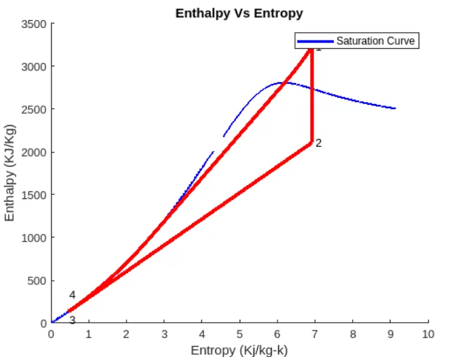
H-S (Enthalpy vs. Entropy) Diagram: Saturation Enthalpy Lines:The blue curves represent lines of constant enthalpy in the two-phase region, connecting the saturated liquid and vapor states. Process Lines (1-2, 2-3, 3-4, 4-5, 5-1): Similar to the T-S diagram, the red lines represent the processes in the Rankine Cycle. Critical Point: The critical point is often noticeable as a point where the saturated liquid and vapor curves meet in the two-phase region.