Project 2 - Rankine cycle Simulator
Project 2 - Rankine cycle Simulator
PROBLEM STATEMENT:-
Understand the concept of Rankine cycle by referring to standard thermal engineering text book.
- Create a Rankine Cycle Simulator using OCTAVE/MATLAB.
- Your code should calculate the state points of the Rankine Cycle (any type of your choice) based on user inputs.
- Then, plot the corresponding T-s and h-s plots for the given set of inputs. Title and axes labels are a must, while legends could be used if necessary.
- The presentation of your code will be taken into consideration while grading. Labelling sections of your code using comments is appreciated.
- Attach a report explaining the working of a rankine cycle simulator and also the research done by you.
Required Inputs:
Turbine Inlet temperature = 400° C
Turbine Inlet Pressure = 30 bars
Turbine Outlet Pressure = 0.05 bars = Condenser Inlet Pressure
Calculate the followings,
- Net work output
- Back work ratio
SOLUTION WITH THE REPORT:-
Lets begin with some Description of the Rankine Cycle.
One of the cycles fueled by vapour is the Rankine cycle. This cycle differs slightly from a gas-powered cycle in that the working fluid was gas the entire time. Steam serves as the working fluid in vapour powered cycles because to its numerous positive qualities, including its availability, low cost of production, and high enthalpy of vaporisation. The Carnot cycle is ideally suited for nuclear power plants and other steam-related power generating sources since it can avoid many practical problems connected with it by superheating the steam and causing it to condense in the condenser.
The process in Rankine cycle are given as:
- Isentropic Compression in Pump.
- Constant pressure heat addition in boiler.
- Isentropic expansion in a turbine.
- Constant pressure heat rejection in condenser.
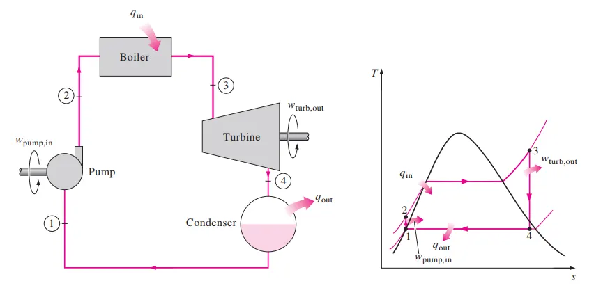
Water enters the pump in state 1 as a saturated liquid and is isentropically compressed to the boiler's operating pressure. Due to a minor reduction in the specific volume of water, the temperature of the water rises a little bit throughout this isentropic compression process. On the T-s figure, the vertical distance between states 1 and 2 has been considerably inflated for clarity.
In stage 2, compressed liquid water enters the boiler. In state 3, superheated vapour exits the boiler. Essentially, the boiler is a sizable heat exchanger where heat from combustion gases, nuclear reactors, or other sources is transported to the water under pressure that is almost constant. The boiler and the area where the steam is superheated (the superheater) are collectively referred to as the steam generator.
The turbine receives the superheated vapour in condition 3, which expands isentropically and generates work by turning a shaft that is attached to an electric generator. During this process, steam loses pressure and heat until it reaches the levels at state 4, when it enters the condenser. Steam is often a high-quality saturated liquid-vapor combination in this stage. In the condenser, which is essentially a giant heat exchanger, steam is condensed at constant pressure by rejecting heat to a cooling medium like a lake, a river, or the atmosphere. The cycle is completed when saturated liquid steam exits the condenser and enters the pump. Power plants are cooled by air rather than water in places where water is scarce.This method of cooling, which is also used in car engines, is called dry cooling.
Keeping in mind that the area under the process curve on a T-s diagram represents the heat transfer for internally reversible processes, we can see that the heat transferred to the water in the boiler is represented by process curve 2-3, and the heat rejected in the condenser is represented by process curve 4-1. The net work generated during the cycle distinguishes these two.
Since all four parts of the Rankine cycle are devices with constant flows, the process using this device may be categorised as a steady state process. The steam mass per unit of steady state flow energy drops to:
`( q I n − q o u t ) + ( W I n − W o u t ) = h e − h i`
The boiler and condenser are not involved in any mechanical work whereas pump and turbine are assumed to isentropic in nature while working throughout the cycle, then conservation of energy relation for each device can be expressed as:
`W p u m p = h 2 − h 1`
where,
`h 1 = h f a t P 1 and v 1 = v f a t P 1`
The heat added in boiler can be given as:
`q I n = h 3 − h 2`
The work which can be taken out of cycle from turbine is given as:
`W o u t = h 3 − h 4`
The heat removed from the condenser is given as:
`q o u t = h 4 − h 1`
The thermal efficiency of Rankine cycle is given as:
`η t h = (W N e t)/ (q I n) = 1 − (q o u t)/ (q I n)`
Where,
`W N e t = q I n − q o u t = W t u r b − W p u m p`
#MATLAB code to run and steup the above problem for the desired solutions:-
clear all
close all
clc

% Rankine Cycle Simulator

fprintf(' Rankine Cycle\n ')
fprintf('1-2 is Isentropic Expansion in Turbine\n')
fprintf(' 2-3 is constant pressure heat removal\n')
fprintf(' 3-4 is Isentropic Compression in Pump \n')
fprintf(' 4-1 Constant pressure Heat addition in Boiler\n')

% Entering the input data for calculation of state points
p1 = 50;        %Pressure at Turbine Inlet
T1 = 500;       %Temperature at Turbine Inlet
p2 = 5;      %Pressure at Condenser

% Taking data from Xsteam file for State point 1
h1 = XSteam('h_pT', p1, T1);        % Enthaply at pressure and Temp 1
s1 = XSteam('s_pT', p1, T1);        % Entropy at pressure and Temp 1

% Taking data from Xsteam file for State point 2
s2 = s1;                            % Because of Isentropic Expansion
sf2 = XSteam('sL_p', p2);           % Saturated liquid entropy at pressure 2
sg2 = XSteam('sV_p', p2);           % Saturated vapour entropy at pressure 2
x2 = (s2-sf2)/(sg2-sf2);            % Vapour Fraction at state point 2
hf2 = XSteam('hL_p', p2);           % Saturated liquid Enthalpy at pressure 2
hg2 = XSteam('hV_p', p2);           % Saturated vapour Enthalpy at pressure 2
h2 = hf2 + (x2*(hg2-hf2));          % Enthalpy at state point 2

% Taking data from Xsteam file for state point 3
p3 = p2;                            % Constant Pressure heat removal process
s3 = XSteam('sL_p', p3);            % Saturated liquid entropy at Pressure 3
h3 = XSteam('hL_p', p3);            % Saturated liquid Enthalpy at Pressure 3

% Taking data from Xsteam file for State point 4
s4 = s3;                            % Isentropic Compression process
p4 = p1;                            % Constant Pressure heat rejection

% Work done in Turbine for the rankine cycle
W_T = h1-h2;

% Work done required for pump
v3 = XSteam('vL_p',p3);             % Saturated Liquid Vapour at pressure 3
W_P = v3*(p4-p3)*100;               % Work done for pump
h4 = h3 - W_P;                      % Enthalpy at State point 4

% Net work done for Rankine Cycle
W_net = W_T - W_P;

% Heat Addition to System
Q_in = h1-h4;

% Heat Rejection from System
Q_out = h2-h3;

% Thermal Efficiency of Rankine Cycle
T_eff = (W_net/Q_in)*100;

%specific steam consumption  = (Mass flow rate / Net work done)
Sp_S = (3600/W_net);

% Calculation of Temperature at All state Point 2, 3 and 4
T3 = XSteam('Tsat_p',p3);           % Saturation Temperature at Pressure 3
T2 = T3;                            % Becuase of Constant Pressure Heat addition
Cp4 = XSteam('Cp_ps',p4,s4);        % Specific isobaric heat capacity
Cv4 = XSteam('Cv_ps',p4,s4);        % Specific isochoric heat capacity
k = Cp4/Cv4;
T4 = T3/((p3/p4)^((k-1)/k));        % Temperature at State point 4

% Calculation of Other constant for saturated liquid and Vapour
T6 = XSteam('Tsat_p', p1);          % Saturated Temperature at Pressure 1
s5 = XSteam('sL_p', p1);            % Saturated Liquid entropy at pressure 1
s6 = XSteam('sV_p', p1);            % Saturated Vapour entropy at Pressure 1
h5 = XSteam('hL_p', p1);            % Saturated Liquid Enthalpy at Pressure 1
h6 = XSteam('hV_p', p1);            % Saturated Vapour Enthalpy at pressure 1
T5 = T6;

%Plotting for Saturation Line
T = linspace(1,560,1000);
for i = 1:length(T)
    sf(i) = XSteam('sL_T' ,T(i));   % Saturated Liquid Entropy
    sg(i) = XSteam('sV_T' ,T(i));   % Saturated Vapour Entropy
    hf(i) = XSteam('hL_T' ,T(i));   % Saturated Liquid Enthalpy
    hg(i) = XSteam('hV_T' ,T(i));   % Saturated Vapour Enthalpy

end

% Plotting T-S Diagram for Rankine Cycle
figure(1)
hold on
plot(sf,T,'color','b','linewidth',2)
plot(sg,T,'color','b','linewidth',2)
plot([s1 s2],[T1 T2], 'color', 'r', 'linewidth',3)
plot([s2 s3],[T2 T3], 'color', 'r', 'linewidth',3)
plot([s3 s4],[T3 T4], 'color', 'r', 'linewidth',3)
plot([s4 s5],[T4 T5], 'color', 'r', 'linewidth',3)
plot([s5 s6],[T5 T6], 'color', 'r', 'linewidth',3)
s_1 = linspace(s6,s1,1000);
for j = 1:length(s_1)
    Tc(j) = XSteam('T_ps',p1,s_1(j));
end

plot(s_1,Tc,'color','r','linewidth',3)
text(s1+0.1, T1, '1')
text(s2+0.1, T2, '2')
text(s3, T3-20, '3')
text(s4, T4+20, '4')
title('Temperature Vs Entropy')
xlabel('Entropy (Kj/kg-k)')
ylabel('Temeperature (Deg. Celcius)')
legend('Saturation Curve')

% Plotting H-S Diagram for Rankine Cycle
figure(2)
hold on
plot(sf,hf,'color','b','linewidth',2)
plot(sg,hg,'color','b','linewidth',2)
plot([s1 s2],[h1 h2],'color','r','linewidth',3)
plot([s2 s3],[h2 h3],'color','r','linewidth',3)
plot([s3 s4],[h3 h4],'color','r','linewidth',3)
hc = linspace(h4,h5,100);
for k = 1:length(hc)
    s_c(k) = XSteam('s_ph',p1,hc(k));
end
plot(s_c,hc,'color','r','linewidth',3)
plot([s5 s6],[h5 h6],'color','r','linewidth',3)
for l = 1:length(s_1)
    h_c(l) = XSteam('h_ps',p1,s_1(l));
end

plot(s_1,h_c,'color','r','linewidth',3)
text(s1+0.1,h1,'1')
text(s2+0.1,h2,'2')
text(s3,h3-100,'3')
text(s4,h4+200,'4')
title('Enthalpy Vs Entropy')
xlabel('Entropy (Kj/kg-k)')
ylabel('Enthalpy (KJ/Kg)')
legend('Saturation Curve')

% Displaying Results in Command window
disp('Results of Rankine Cycle')
fprintf('At state point 1\t\t\t\t\t')
fprintf('At state Point 2\n')
fprintf('P1 = %10f in Bar\t\t\t\t',p1);
fprintf('P2 = %10f in Bar\n',p2);
fprintf('T1 = %11f in Deg.Celcius\t\t',T1);
fprintf('T2 = %11f in Deg.Celcius\n',T2);
fprintf('H1 = %12f in KJ/Kg\t\t\t',h1);
fprintf('H2 = %12f in KJ/Kg\n',h2);
fprintf('S1 = %9f in KJ/Kg-k\t\t\t',s1);
fprintf('S2 = %9f in KJ/Kg-k\n',s2);
fprintf('\n')
fprintf('At state point 3\t\t\t\t\t')
fprintf('At state Point 4\n')
fprintf('P3 = %10f in Bar\t\t\t\t',p3);
fprintf('P4 = %10f in Bar\n',p4);
fprintf('T3 = %11f in Deg.Celcius\t\t',T3);
fprintf('T4 = %11f in Deg.Celcius\n',T4);
fprintf('H3 = %12f in KJ/Kg\t\t\t',h3);
fprintf('H4 = %12f in KJ/Kg\n',h4);
fprintf('S3 = %9f in KJ/Kg-k\t\t\t',s3);
fprintf('S4 = %9f in KJ/Kg-k\n',s4);
fprintf('\n')
fprintf('Turbine Work Done = %14f in KJ/Kg\n',W_T)
fprintf('Pump Work Done = %15f in KJ/Kg\n',W_P)
fprintf('Net Work Done  = %17f in KJ/Kg\n',W_net)
fprintf('Thermal Efficiency = %13f in percent\n',T_eff)
fprintf('Sp. Steam Consumption = %f in KJ/Kw\n',Sp_S)
Explanation of the above code:-
This MATLAB code simulates and analyzes the Rankine cycle, a thermodynamic cycle commonly used in steam power plants. The Rankine cycle is used to model the behavior of a steam turbine-based power generation system. The script calculates various thermodynamic properties and then uses them to plot temperature-entropy (T-S) and enthalpy-entropy (H-S) diagrams for the cycle. Additionally, it displays the results in the command window.
clear all
close all
clc
These lines clear the workspace, close all open figures, and clear the command window.
fprintf(' Rankine Cycle\n ')
fprintf('1-2 is Isentropic Expansion in Turbine\n')
fprintf(' 2-3 is constant pressure heat removal\n')
fprintf(' 3-4 is Isentropic Compression in Pump \n')
fprintf(' 4-1 Constant pressure Heat addition in Boiler\n')
These lines use the fprintf function to display information about the different processes in the Rankine cycle.
p1 = 70;         % Pressure at Turbine Inlet
T1 = 700;        % Temperature at Turbine Inlet
p2 = 7;          % Pressure at Condenser
Here, pressure p1 and temperature T1 are defined as the initial conditions for the turbine inlet, and pressure p2 is set as the pressure at the condenser.
h1 = XSteam('h_pT', p1, T1);        % Enthalpy at pressure and Temp 1
s1 = XSteam('s_pT', p1, T1);        % Entropy at pressure and Temp 1
These lines use the XSteam function to obtain the enthalpy (h1) and entropy (s1) values at state point 1 based on the given pressure and temperature.
s2 = s1;                            % Because of Isentropic Expansion
sf2 = XSteam('sL_p', p2);           % Saturated liquid entropy at pressure 2
sg2 = XSteam('sV_p', p2);           % Saturated vapor entropy at pressure 2
x2 = (s2 - sf2) / (sg2 - sf2);      % Vapor Fraction at state point 2
hf2 = XSteam('hL_p', p2);           % Saturated liquid Enthalpy at pressure 2
hg2 = XSteam('hV_p', p2);           % Saturated vapor Enthalpy at pressure 2
h2 = hf2 + (x2 * (hg2 - hf2));      % Enthalpy at state point 2
These lines calculate properties at state point 2, including entropy (s2), vapor fraction (x2), and enthalpy (h2), based on isentropic expansion assumptions.
p3 = p2;                            % Constant Pressure heat removal process
s3 = XSteam('sL_p', p3);            % Saturated liquid entropy at Pressure 3
h3 = XSteam('hL_p', p3);            % Saturated liquid Enthalpy at Pressure 3
These lines set the pressure at state point 3 (p3) and then calculate the corresponding properties (s3 and h3) based on saturated liquid assumptions.
s4 = s3;                            % Isentropic Compression process
p4 = p1;                            % Constant Pressure heat rejection
Here, entropy at state point 4 (s4) is set equal to the entropy at state point 3, assuming isentropic compression. Pressure at state point 4 (p4) is set equal to the pressure at the turbine inlet.
W_T = h1 - h2;                      % Work done in Turbine for the Rankine cycle
v3 = XSteam('vL_p', p3);             % Saturated Liquid Volume at pressure 3
W_P = v3 * (p4 - p3) * 100;          % Work done for pump
h4 = h3 - W_P;                       % Enthalpy at State point 4
These lines calculate the work done in the turbine (W_T), the work done by the pump (W_P), and the resulting enthalpy at state point 4 (h4).
W_net = W_T - W_P;                  % Net work done for Rankine Cycle
Q_in = h1 - h4;                      % Heat Addition to System
Q_out = h2 - h3;                     % Heat Rejection from System
T_eff = (W_net / Q_in) * 100;        % Thermal Efficiency of Rankine Cycle
Sp_S = (3600 / W_net);               % Specific steam consumption
These lines calculate the net work done (W_net), heat addition (Q_in), heat rejection (Q_out), thermal efficiency (T_eff), and specific steam consumption (Sp_S) for the Rankine cycle.
Inference of Plot:
To make the graph more deliberate we are changing some value in the inputs by increasing the inlet pressure and temperature along with condenser pressure also which results in following graphs
Results of the above inputs,
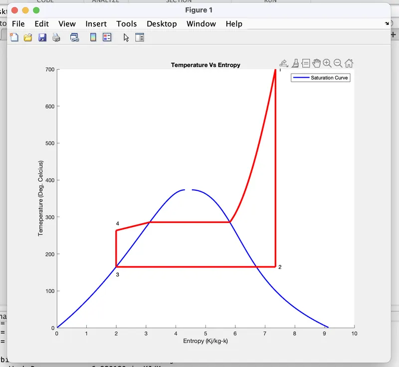
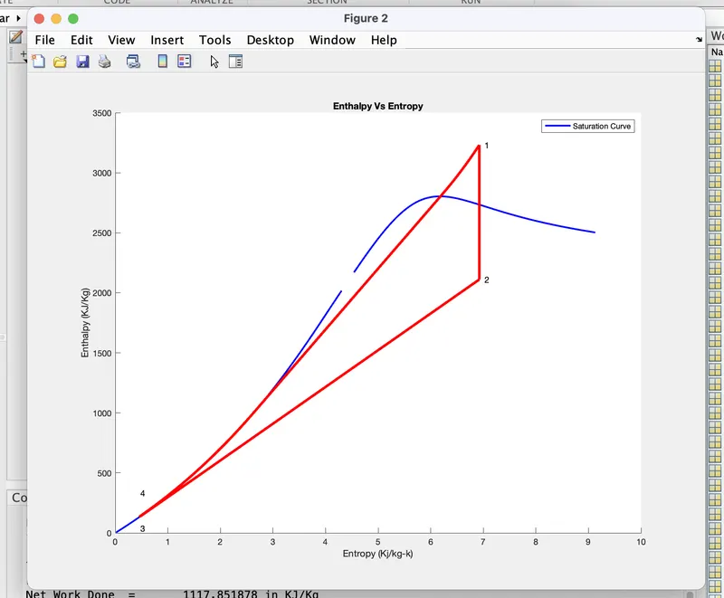
As we can see from the above figure, point 1 begins with a turbine from which heat rejection is initiated, which is once more an isentropic process. As the steam is beneath the curve, it cools in the condenser and becomes a saturated liquid. It was then fed into a boiler, where its temperature was raised to convert it from a saturated liquid to vapour.
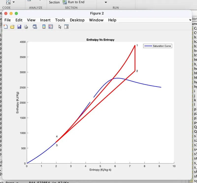
The accompanying graphic shows how the steam's entropy varies in relation to enthalpy during the procedure. Entropy has grown as heat has been introduced to the system, and it has decreased at about the same rates as heat has been withdrawn.
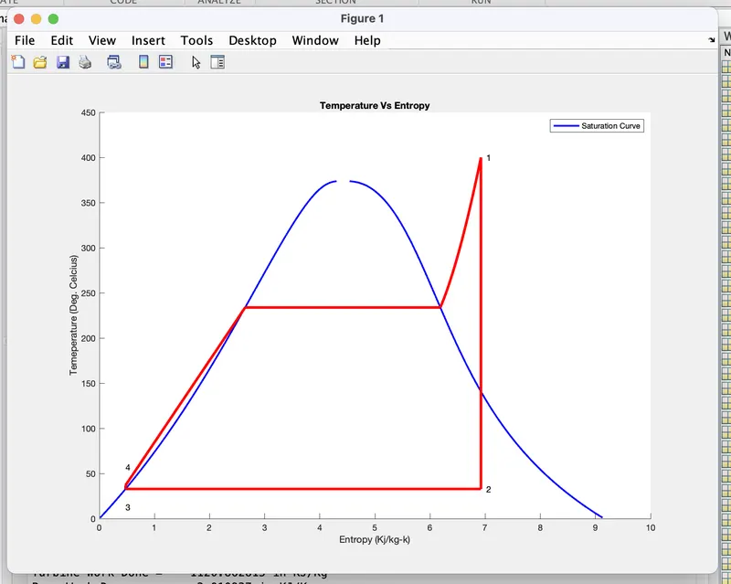
For the Parameters given in the challenge the graph will look like this:-
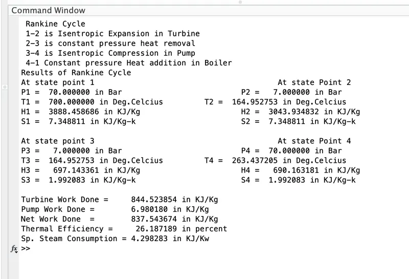
The values for the state point in command windows are given as:
For Inlet pressure in Turbine as = 70 bar
Inlet temperature in Turbine = 700 deg.cel
Pressure in condenser = 7 bar
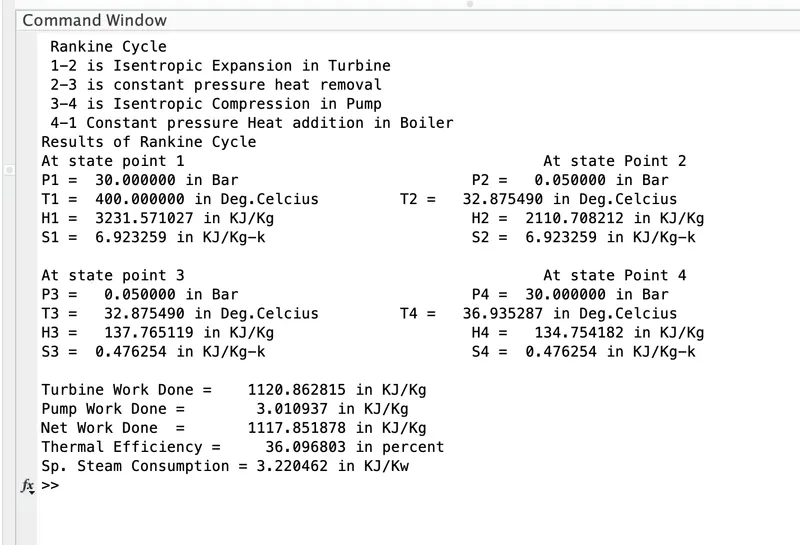
For Inputs given in challenge:
For Inlet pressure in Turbine as = 30 bar
Inlet temperature in Turbine = 400 deg.cel
Pressure in condenser = 0.05 bar
CONCLUSIONS:-
From the two different input value it is seen that increasing the pressure and temperature in turbine result in lowering the efficiency of Rankine cycle.As a result, we developed the Rankine cycle simulator for the provided input, using data from the XSteam function file.