Project 2
Binary Search
In this tutorial, you will learn how Binary Search sort works. Also, you will find working examples of Binary Search in C, C++, Java and Python.
Binary Search is a searching algorithm for finding an element's position in a sorted array.
In this approach, the element is always searched in the middle of a portion of an array.
Binary search can be implemented only on a sorted list of items. If the elements are not sorted already, we need to sort them first.
Binary Search Working
Binary Search Algorithm can be implemented in two ways which are discussed below.
- Iterative Method
- Recursive Method
The recursive method follows the divide and conquer approach.
The general steps for both methods are discussed below.
- The array in which searching is to be performed is:
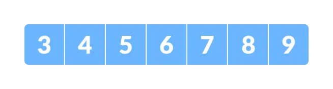
Initial array
Letx = 4be the element to be searched. - Set two pointers low and high at the lowest and the highest positions respectively.
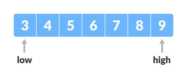
Setting pointers - Find the middle element mid of the array ie.
arr[(low + high)/2] = 6.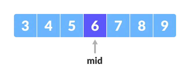
Mid element - If x == mid, then return mid.Else, compare the element to be searched with m.
- If
x > mid, compare x with the middle element of the elements on the right side of mid. This is done by setting low tolow = mid + 1. - Else, compare x with the middle element of the elements on the left side of mid. This is done by setting high to
high = mid - 1.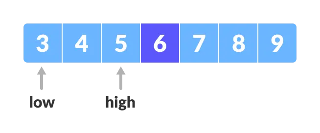
Finding mid element - Repeat steps 3 to 6 until low meets high.
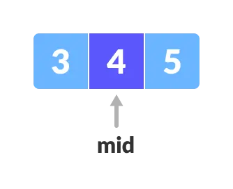
Mid element x = 4is found.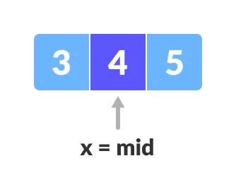
Found
Binary Search Algorithm
Iteration Method
do until the pointers low and high meet each other.
    mid = (low + high)/2
    if (x == arr[mid])
        return mid
    else if (x > arr[mid]) // x is on the right side
        low = mid + 1
    else                       // x is on the left side
        high = mid - 1
Recursive Method
binarySearch(arr, x, low, high)
    if low > high
        return False
    else
        mid = (low + high) / 2
        if x == arr[mid]
            return mid
        else if x > arr[mid]        // x is on the right side
            return binarySearch(arr, x, mid + 1, high)
        else                               // x is on the right side
            return binarySearch(arr, x, low, mid - 1)
Python, Java, C/C++ Examples (Iterative Method)
# Binary Search in python


def binarySearch(array, x, low, high):

    # Repeat until the pointers low and high meet each other
    while low <= high:

        mid = low + (high - low)//2

        if array[mid] == x:
            return mid

        elif array[mid] < x:
            low = mid + 1

        else:
            high = mid - 1

    return -1


array = [3, 4, 5, 6, 7, 8, 9]
x = 4

result = binarySearch(array, x, 0, len(array)-1)

if result != -1:
joined LinkedIn about six years ago at a particularly interesting time. We were just beginning to run up against the limits of our monolithic, centralized database and needed to start the transition to a portfolio of specialized distributed systems. This has been an interesting experience: we built, deployed, and run to this day a distributed graph database, a distributed search backend, a Hadoop installation, and a first and second generation key-value store.
One of the most useful things I learned in all this was that many of the things we were building had a very simple concept at their heart: the log. Sometimes called write-ahead logs or commit logs or transaction logs, logs have been around almost as long as computers and are at the heart of many distributed data systems and real-time application architectures.
You can't fully understand databases, NoSQL stores, key value stores, replication, paxos, hadoop, version control, or almost any software system without understanding logs; and yet, most software engineers are not familiar with them. I'd like to change that. In this post, I'll walk you through everything you need to know about logs, including what is log and how to use logs for data integration, real time processing, and system building.
Part One: What Is a Log?
A log is perhaps the simplest possible storage abstraction. It is an append-only, totally-ordered sequence of records ordered by time. It looks like this:
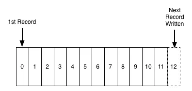
Records are appended to the end of the log, and reads proceed left-to-right. Each entry is assigned a unique sequential log entry number.
The ordering of records defines a notion of "time" since entries to the left are defined to be older then entries to the right. The log entry number can be thought of as the "timestamp" of the entry. Describing this ordering as a notion of time seems a bit odd at first, but it has the convenient property that it is decoupled from any particular physical clock. This property will turn out to be essential as we get to distributed systems.
The contents and format of the records aren't important for the purposes of this discussion. Also, we can't just keep adding records to the log as we'll eventually run out of space. I'll come back to this in a bit.
So, a log is not all that different from a file or a table. A file is an array of bytes, a table is an array of records, and a log is really just a kind of table or file where the records are sorted by time.
At this point you might be wondering why it is worth talking about something so simple? How is a append-only sequence of records in any way related to data systems? The answer is that logs have a specific purpose: they record what happened and when. For distributed data systems this is, in many ways, the very heart of the problem.
But before we get too far let me clarify something that is a bit confusing. Every programmer is familiar with another definition of logging—the unstructured error messages or trace info an application might write out to a local file using syslog or log4j. For clarity I will call this "application logging". The application log is a degenerative form of the log concept I am describing. The biggest difference is that text logs are meant to be primarily for humans to read and the "journal" or "data logs" I'm describing are built for programmatic access.
(Actually, if you think about it, the idea of humans reading through logs on individual machines is something of an anachronism. This approach quickly becomes an unmanageable strategy when many services and servers are involved and the purpose of logs quickly becomes as an input to queries and graphs to understand behavior across many machines—something for which english text in files is not nearly as appropriate as the kind structured log described here.)
Logs in databases
I don't know where the log concept originated—probably it is one of those things like binary search that is too simple for the inventor to realize it was an invention. It is present as early as IBM's System R. The usage in databases has to do with keeping in sync the variety of data structures and indexes in the presence of crashes. To make this atomic and durable, a database uses a log to write out information about the records they will be modifying, before applying the changes to all the various data structures it maintains. The log is the record of what happened, and each table or index is a projection of this history into some useful data structure or index. Since the log is immediately persisted it is used as the authoritative source in restoring all other persistent structures in the event of a crash.
Over-time the usage of the log grew from an implementation detail of ACID to a method for replicating data between databases. It turns out that the sequence of changes that happened on the database is exactly what is needed to keep a remote replica database in sync. Oracle, MySQL, and PostgreSQL include log shipping protocols to transmit portions of log to replica databases which act as slaves. Oracle has productized the log as a general data subscription mechanism for non-oracle data subscribers with their XStreamsand GoldenGate and similar facilities in MySQL and PostgreSQL are key components of many data architectures.
Because of this origin, the concept of a machine readable log has largely been confined to database internals. The use of logs as a mechanism for data subscription seems to have arisen almost by chance. But this very abstraction is ideal for supporting all kinds of messaging, data flow, and real-time data processing.
Logs in distributed systems
The two problems a log solves—ordering changes and distributing data—are even more important in distributed data systems. Agreeing upon an ordering for updates (or agreeing to disagree and coping with the side-effects) are among the core design problems for these systems.
The log-centric approach to distributed systems arises from a simple observation that I will call the State Machine Replication Principle:
This may seem a bit obtuse, so let's dive in and understand what it means.
Deterministic means that the processing isn't timing dependent and doesn't let any other "out of band" input influence its results. For example a program whose output is influenced by the particular order of execution of threads or by a call to gettimeofday or some other non-repeatable thing is generally best considered as non-deterministic.
The state of the process is whatever data remains on the machine, either in memory or on disk, at the end of the processing.
The bit about getting the same input in the same order should ring a bell—that is where the log comes in. This is a very intuitive notion: if you feed two deterministic pieces of code the same input log, they will produce the same output.
The application to distributed computing is pretty obvious. You can reduce the problem of making multiple machines all do the same thing to the problem of implementing a distributed consistent log to feed these processes input. The purpose of the log here is to squeeze all the non-determinism out of the input stream to ensure that each replica processing this input stays in sync.
When you understand it, there is nothing complicated or deep about this principle: it more or less amounts to saying "deterministic processing is deterministic". Nonetheless, I think it is one of the more general tools for distributed systems design.
One of the beautiful things about this approach is that the time stamps that index the log now act as the clock for the state of the replicas—you can describe each replica by a single number, the timestamp for the maximum log entry it has processed. This timestamp combined with the log uniquely captures the entire state of the replica.
There are a multitude of ways of applying this principle in systems depending on what is put in the log. For example, we can log the incoming requests to a service, or the state changes the service undergoes in response to request, or the transformation commands it executes. Theoretically, we could even log a series of machine instructions for each replica to execute or the method name and arguments to invoke on each replica. As long as two processes process these inputs in the same way, the processes will remaining consistent across replicas.
Different groups of people seem to describe the uses of logs differently. Database people generally differentiate between physical and logical logging. Physical logging means logging the contents of each row that is changed. Logical logging means logging not the changed rows but the SQL commands that lead to the row changes (the insert, update, and delete statements).
The distributed systems literature commonly distinguishes two broad approaches to processing and replication. The "state machine model" usually refers to an active-active model where we keep a log of the incoming requests and each replica processes each request. A slight modification of this, called the "primary-backup model", is to elect one replica as the leader and allow this leader to process requests in the order they arrive and log out the changes to its state from processing the requests. The other replicas apply in order the state changes the leader makes so that they will be in sync and ready to take over as leader should the leader fail.
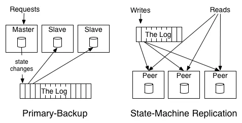
To understand the difference between these two approaches, let's look at a toy problem. Consider a replicated "arithmetic service" which maintains a single number as its state (initialized to zero) and applies additions and multiplications to this value. The active-active approach might log out the transformations to apply, say "+1", "*2", etc. Each replica would apply these transformations and hence go through the same set of values. The "active-passive" approach would have a single master execute the transformations and log out the result, say "1", "3", "6", etc. This example also makes it clear why ordering is key for ensuring consistency between replicas: reordering an addition and multiplication will yield a different result.
 The distributed log can be seen as the data structure which models the problem of consensus. A log, after all, represents a series of decisions on the "next" value to append. You have to squint a little to see a log in the Paxos family of algorithms, though log-building is their most common practical application. With Paxos, this is usually done using an extension of the protocol called "multi-paxos", which models the log as a series of consensus problems, one for each slot in the log. The log is much more prominent in other protocols such as ZAB, RAFT, and Viewstamped Replication, which directly model the problem of maintaining a distributed, consistent log.
My suspicion is that our view of this is a little bit biased by the path of history, perhaps due to the few decades in which the theory of distributed computing outpaced its practical application. In reality, the consensus problem is a bit too simple. Computer systems rarely need to decide a single value, they almost always handle a sequence of requests. So a log, rather than a simple single-value register, is the more natural abstraction.
Furthermore, the focus on the algorithms obscures the underlying log abstraction systems need. I suspect we will end up focusing more on the log as a commoditized building block irrespective of its implementation in the same way we often talk about a hash table without bothering to get in the details of whether we mean the murmur hash with linear probing or some other variant. The log will become something of a commoditized interface, with many algorithms and implementations competing to provide the best guarantees and optimal performance.
Changelog 101: Tables and Events are Dual
Let's come back to databases for a bit. There is a facinating duality between a log of changes and a table. The log is similar to the list of all credits and debits and bank processes; a table is all the current account balances. If you have a log of changes, you can apply these changes in order to create the table capturing the current state. This table will record the latest state for each key (as of a particular log time). There is a sense in which the log is the more fundamental data structure: in addition to creating the original table you can also transform it to create all kinds of derived tables. (And yes, table can mean keyed data store for the non-relational folks.) 
This process works in reverse too: if you have a table taking updates, you can record these changes and publish a "changelog" of all the updates to the state of the table. This changelog is exactly what you need to support near-real-time replicas. So in this sense you can see tables and events as dual: tables support data at rest and logs capture change. The magic of the log is that if it is a completelog of changes, it holds not only the contents of the final version of the table, but also allows recreating all other versions that might have existed. It is, effectively, a sort of backup of every previous state of the table.
This might remind you of source code version control. There is a close relationship between source control and databases. Version control solves a very similar problem to what distributed data systems have to solve—managing distributed, concurrent changes in state. A version control system usually models the sequence of patches, which is in effect a log. You interact directly with a checked out "snapshot" of the current code which is analogous to the table. You will note that in version control systems, as in other distributed stateful systems, replication happens via the log: when you update, you pull down just the patches and apply them to your current snapshot.
Some people have seen some of these ideas recently from Datomic, a company selling a log-centric database. This presentation gives a great overview of how they have applied the idea in their system. These ideas are not unique to this system, of course, as they have been a part of the distributed systems and database literature for well over a decade.
This may all seem a little theoretical. Do not despair! We'll get to practical stuff pretty quickly.
What's next
In the remainder of this article I will try to give a flavor of what a log is good for that goes beyond the internals of distributed computing or abstract distributed computing models. This includes:
- Data Integration—Making all of an organization's data easily available in all its storage and processing systems.
- Real-time data processing—Computing derived data streams.
- Distributed system design—How practical systems can by simplified with a log-centric design.
These uses all resolve around the idea of a log as a stand-alone service.
In each case, the usefulness of the log comes from simple function that the log provides: producing a persistent, re-playable record of history. Surprisingly, at the core of these problems is the ability to have many machines playback history at their own rate in a deterministic manner.
Part Two: Data Integration
Let me first say what I mean by "data integration" and why I think it's important, then we'll see how it relates back to logs.
This phrase "data integration" isn't all that common, but I don't know a better one. The more recognizable term ETL usually covers only a limited part of data integration—populating a relational data warehouse. But much of what I am describing can be thought of as ETL generalized to cover real-time systems and processing flows. 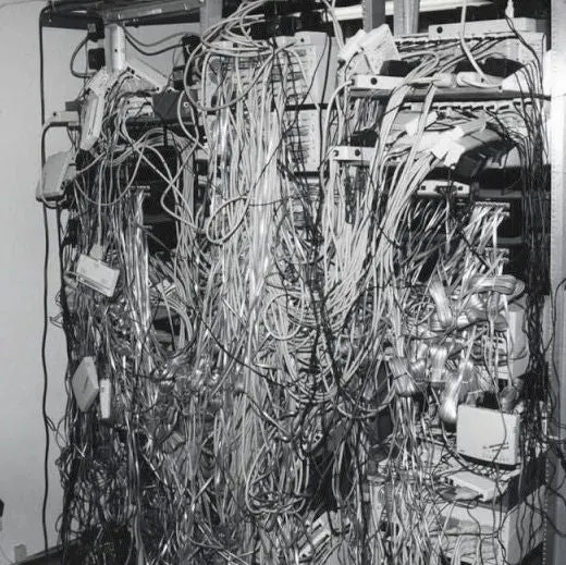
You don't hear much about data integration in all the breathless interest and hype around the idea of big data, but nonetheless, I believe this mundane problem of "making the data available" is one of the more valuable things an organization can focus on.
Effective use of data follows a kind of Maslow's hierarchy of needs. The base of the pyramid involves capturing all the relevant data, being able to put it together in an applicable processing environment (be that a fancy real-time query system or just text files and python scripts). This data needs to be modeled in a uniform way to make it easy to read and process. Once these basic needs of capturing data in a uniform way are taken care of it is reasonable to work on infrastructure to process this data in various ways—MapReduce, real-time query systems, etc.
It's worth noting the obvious: without a reliable and complete data flow, a Hadoop cluster is little more than a very expensive and difficult to assemble space heater. Once data and processing are available, one can move concern on to more refined problems of good data models and consistent well understood semantics. Finally, concentration can shift to more sophisticated processing—better visualization, reporting, and algorithmic processing and prediction.
In my experience, most organizations have huge holes in the base of this pyramid—they lack reliable complete data flow—but want to jump directly to advanced data modeling techniques. This is completely backwards.
So the question is, how can we build reliable data flow throughout all the data systems in an organization?
Data Integration: Two complications
Two trends make data integration harder.
The event data firehose
The first trend is the rise of event data. Event data records things that happen rather than things that are. In web systems, this means user activity logging, but also the machine-level events and statistics required to reliably operate and monitor a data center's worth of machines. People tend to call this "log data" since it is often written to application logs, but that confuses form with function. This data is at the heart of the modern web: Google's fortune, after all, is generated by a relevance pipeline built on clicks and impressions—that is, events.
And this stuff isn't limited to web companies, it's just that web companies are already fully digital, so they are easier to instrument. Financial data has long been event-centric. RFID adds this kind of tracking to physical objects. I think this trend will continue with the digitization of traditional businesses and activities.
This type of event data records what happened, and tends to be several orders of magnitude larger than traditional database uses. This presents significant challenges for processing.
The explosion of specialized data systems
The second trend comes from the explosion of specialized data systems that have become popular and often freely available in the last five years. Specialized systems exist for OLAP, search, simple online storage, batch processing, graph analysis, and so on.
The combination of more data of more varieties and a desire to get this data into more systems leads to a huge data integration problem.
Log-structured data flow
The log is the natural data structure for handling data flow between systems. The recipe is very simple:
Each logical data source can be modeled as its own log. A data source could be an application that logs out events (say clicks or page views), or a database table that accepts modifications. Each subscribing system reads from this log as quickly as it can, applies each new record to its own store, and advances its position in the log. Subscribers could be any kind of data system—a cache, Hadoop, another database in another site, a search system, etc. 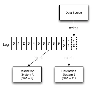
For example, the log concept gives a logical clock for each change against which all subscribers can be measured. This makes reasoning about the state of the different subscriber systems with respect to one another far simpler, as each has a "point in time" they have read up to.
To make this more concrete, consider a simple case where there is a database and a collection of caching servers. The log provides a way to synchronize the updates to all these systems and reason about the point of time of each of these systems. Let's say we write a record with log entry X and then need to do a read from the cache. If we want to guarantee we don't see stale data, we just need to ensure we don't read from any cache which has not replicated up to X.
The log also acts as a buffer that makes data production asynchronous from data consumption. This is important for a lot of reasons, but particularly when there are multiple subscribers that may consume at different rates. This means a subscribing system can crash or go down for maintenance and catch up when it comes back: the subscriber consumes at a pace it controls. A batch system such as Hadoop or a data warehouse may consume only hourly or daily, whereas a real-time query system may need to be up-to-the-second. Neither the originating data source nor the log has knowledge of the various data destination systems, so consumer systems can be added and removed with no change in the pipeline.
Binary search is one of the fundamental algorithms in computer science. In order to explore it, we’ll first build up a theoretical backbone, then use that to implement the algorithm properly and avoid those nasty off-by-one errors everyone’s been talking about.
FINDING A VALUE IN A SORTED SEQUENCE
In its simplest form, binary search is used to quickly find a value in a sorted sequence (consider a sequence an ordinary array for now). We’ll call the sought value the target value for clarity. Binary search maintains a contiguous subsequence of the starting sequence where the target value is surely located. This is called the search space. The search space is initially the entire sequence. At each step, the algorithm compares the median value in the search space to the target value. Based on the comparison and because the sequence is sorted, it can then eliminate half of the search space. By doing this repeatedly, it will eventually be left with a search space consisting of a single element, the target value.
For example, consider the following sequence of integers sorted in ascending order and say we are looking for the number 55:
| 0 | 5 | 13 | 19 | 22 | 41 | 55 | 68 | 72 | 81 | 98 |
We are interested in the location of the target value in the sequence so we will represent the search space as indices into the sequence. Initially, the search space contains indices 1 through 11. Since the search space is really an interval, it suffices to store just two numbers, the low and high indices. As described above, we now choose the median value, which is the value at index 6 (the midpoint between 1 and 11): this value is 41 and it is smaller than the target value. From this we conclude not only that the element at index 6 is not the target value, but also that no element at indices between 1 and 5 can be the target value, because all elements at these indices are smaller than 41, which is smaller than the target value. This brings the search space down to indices 7 through 11:
| 55 | 68 | 72 | 81 | 98 |
Proceeding in a similar fashion, we chop off the second half of the search space and are left with:
| 55 | 68 |
Depending on how we choose the median of an even number of elements we will either find 55 in the next step or chop off 68 to get a search space of only one element. Either way, we conclude that the index where the target value is located is 7.
If the target value was not present in the sequence, binary search would empty the search space entirely. This condition is easy to check and handle. Here is some code to go with the description:
1 2 3 4 5 6 7 8 9 10binary_search(A, target): lo = 1, hi = size(A) while lo <= hi: mid = lo + (hi - lo) / 2 if A[mid] == target: return mid else if A[mid] < target: lo = mid + 1 else : hi = mid - 1 // target was not found
COMPLEXITY
Since each comparison binary search uses halves the search space, we can assert and easily prove that binary search will never use more than (in big-oh notation) O(log N) comparisons to find the target value.
The logarithm is an awfully slowly growing function. In case you’re not aware of just how efficient binary search is, consider looking up a name in a phone book containing a million names. Binary search lets you systematically find any given name using at most 21 comparisons. If you could manage a list containing all the people in the world sorted by name, you could find any person in less than 35 steps. This may not seem feasible or useful at the moment, but we’ll soon fix that.
Note that this assumes that we have random access to the sequence. Trying to use binary search on a container such as a linked list makes little sense and it is better use a plain linear search instead.
BINARY SEARCH IN STANDARD LIBRARIES
C++’s Standard Template Library implements binary search in algorithms lower_bound, upper_bound, binary_search and equal_range, depending exactly on what you need to do. Java has a built-in Arrays.binary_search method for arrays and the .NET Framework has Array.BinarySearch.
You’re best off using library functions whenever possible, since, as you’ll see, implementing binary search on your own can be tricky.
BEYOND ARRAYS: THE DISCRETE BINARY SEARCH
This is where we start to abstract binary search. A sequence (array) is really just a function which associates integers (indices) with the corresponding values. However, there is no reason to restrict our usage of binary search to tangible sequences. In fact, we can use the same algorithm described above on any monotonic function f whose domain is the set of integers. The only difference is that we replace an array lookup with a function evaluation: we are now looking for some x such that f(x) is equal to the target value. The search space is now more formally a subinterval of the domain of the function, while the target value is an element of the codomain. The power of binary search begins to show now: not only do we need at most O(log N) comparisons to find the target value, but we also do not need to evaluate the function more than that many times. Additionally, in this case we aren’t restricted by practical quantities such as available memory, as was the case with arrays.
TAKING IT FURTHER: THE MAIN THEOREM
When you encounter a problem which you think could be solved by applying binary search, you need some way of proving it will work. I will now present another level of abstraction which will allow us to solve more problems, make proving binary search solutions very easy and also help implement them. This part is a tad formal, but don’t get discouraged, it’s not that bad.
Consider a predicate p defined over some ordered set S (the search space). The search space consists of candidate solutions to the problem. In this article, a predicate is a function which returns a boolean value, true or false (we’ll also use yes and no as boolean values). We use the predicate to verify if a candidate solution is legal (does not violate some constraint) according to the definition of the problem.
What we can call the main theorem states that binary search can be used if and only if for all x in S, p(x) implies p(y) for all y > x. This property is what we use when we discard the second half of the search space. It is equivalent to saying that ¬p(x) implies ¬p(y) for all y < x (the symbol ¬ denotes the logical not operator), which is what we use when we discard the first half of the search space. The theorem can easily be proven, although I’ll omit the proof here to reduce clutter.
Behind the cryptic mathematics I am really stating that if you had a yes or no question (the predicate), getting a yes answer for some potential solution x means that you’d also get a yes answer for any element after x. Similarly, if you got a no answer, you’d get a no answer for any element before x. As a consequence, if you were to ask the question for each element in the search space (in order), you would get a series of no answers followed by a series of yes answers.
Careful readers may note that binary search can also be used when a predicate yields a series of yes answers followed by a series of no answers. This is true and complementing that predicate will satisfy the original condition. For simplicity we’ll deal only with predicates described in the theorem.
If the condition in the main theorem is satisfied, we can use binary search to find the smallest legal solution, i.e. the smallest x for which p(x) is true. The first part of devising a solution based on binary search is designing a predicate which can be evaluated and for which it makes sense to use binary search: we need to choose what the algorithm should find. We can have it find either the first x for which p(x) is true or the last x for which p(x) is false. The difference between the two is only slight, as you will see, but it is necessary to settle on one. For starters, let us seek the first yes answer (first option).
The second part is proving that binary search can be applied to the predicate. This is where we use the main theorem, verifying that the conditions laid out in the theorem are satisfied. The proof doesn’t need to be overly mathematical, you just need to convince yourself that p(x) implies p(y) for all y > x or that ¬p(x) implies ¬p(y) for all y < x. This can often be done by applying common sense in a sentence or two.
When the domain of the predicate are the integers, it suffices to prove that p(x) implies p(x+1) or that ¬p(x) implies ¬p(x-1), the rest then follows by induction.
These two parts are most often interleaved: when we think a problem can be solved by binary search, we aim to design the predicate so that it satisfies the condition in the main theorem.
One might wonder why we choose to use this abstraction rather than the simpler-looking algorithm we’ve used so far. This is because many problems can’t be modeled as searching for a particular value, but it’s possible to define and evaluate a predicate such as “Is there an assignment which costs x or less?”, when we’re looking for some sort of assignment with the lowest cost. For example, the usual traveling salesman problem (TSP) looks for the cheapest round-trip which visits every city exactly once. Here, the target value is not defined as such, but we can define a predicate “Is there a round-trip which costs x or less?” and then apply binary search to find the smallest x which satisfies the predicate. This is called reducing the original problem to a decision (yes/no) problem. Unfortunately, we know of no way of efficiently evaluating this particular predicate and so the TSP problem isn’t easily solved by binary search, but many optimization problems are.
Let us now convert the simple binary search on sorted arrays described in the introduction to this abstract definition. First, let’s rephrase the problem as: “Given an array A and a target value, return the index of the first element in A equal to or greater than the target value.” Incidentally, this is more or less how lower_bound behaves in C++.
We want to find the index of the target value, thus any index into the array is a candidate solution. The search space S is the set of all candidate solutions, thus an interval containing all indices. Consider the predicate “Is A[x] greater than or equal to the target value?”. If we were to find the first x for which the predicate says yes, we’d get exactly what decided we were looking for in the previous paragraph.
The condition in the main theorem is satisfied because the array is sorted in ascending order: if A[x] is greater than or equal to the target value, all elements after it are surely also greater than or equal to the target value.
If we take the sample sequence from before:
| 0 | 5 | 13 | 19 | 22 | 41 | 55 | 68 | 72 | 81 | 98 |
With the search space (indices):
| 1 | 2 | 3 | 4 | 5 | 6 | 7 | 8 | 9 | 10 | 11 |
And apply our predicate (with a target value of 55) to it we get:
| no | no | no | no | no | no | yes | yes | yes | yes | yes |
This is a series of no answers followed by a series of yes answers, as we were expecting. Notice how index 7 (where the target value is located) is the first for which the predicate yields yes, so this is what our binary search will find.
IMPLEMENTING THE DISCRETE ALGORITHM
One important thing to remember before beginning to code is to settle on what the two numbers you maintain (lower and upper bound) mean. A likely answer is a closed interval which surely contains the first x for which p(x) is true. All of your code should then be directed at maintaining this invariant: it tells you how to properly move the bounds, which is where a bug can easily find its way in your code, if you’re not careful.
Another thing you need to be careful with is how high to set the bounds. By “high” I really mean “wide” since there are two bounds to worry about. Every so often it happens that a coder concludes during coding that the bounds he or she set are wide enough, only to find a counterexample during intermission (when it’s too late). Unfortunately, little helpful advice can be given here other than to always double- and triple-check your bounds! Also, since execution time increases logarithmically with the bounds, you can always set them higher, as long as it doesn’t break the evaluation of the predicate. Keep your eye out for overflow errors all around, especially in calculating the median.
Now we finally get to the code which implements binary search as described in this and the previous section:
1 2 3 4 5 6 7 8 9 10 11binary_search(lo, hi, p): while lo < hi: mid = lo + (hi - lo) / 2 if p(mid) == true: hi = mid else : lo = mid + 1 if p(lo) == false: complain // p(x) is false for all x in S! return lo // lo is the least x for which p(x) is true
The two crucial lines are hi = mid and lo = mid+1. When p(mid) is true, we can discard the second half of the search space, since the predicate is true for all elements in it (by the main theorem). However, we can not discard mid itself, since it may well be the first element for which p is true. This is why moving the upper bound to mid is as aggressive as we can do without introducing bugs.
In a similar vein, if p(mid) is false, we can discard the first half of the search space, but this time including mid. p(mid) is false so we don’t need it in our search space. This effectively means we can move the lower bound to mid+1.
If we wanted to find the last x for which p(x) is false, we would devise (using a similar rationale as above) something like:
1 2 3 4 5 6 7 8 9 10 11 12 13// warning: there is a nasty bug in this snippet! binary_search(lo, hi, p): while lo < hi: mid = lo + (hi - lo) / 2 // note: division truncates if p(mid) == true: hi = mid - 1 else : lo = mid if p(lo) == true: complain // p(x) is true for all x in S! return lo // lo is the greatest x for which p(x) is false
You can verify that this satisfies our condition that the element we’re looking for always be present in the interval (lo, hi). However, there is another problem. Consider what happens when you run this code on some search space for which the predicate gives:
| no | yes |
The code will get stuck in a loop. It will always select the first element as mid, but then will not move the lower bound because it wants to keep the no in its search space. The solution is to change mid = lo + (hi-lo)/2 to mid = lo + (hi-lo+1)/2, i.e. so that it rounds up instead of down. There are other ways of getting around the problem, but this one is possibly the cleanest. Just remember to always test your code on a two-element set where the predicate is false for the first element and true for the second.
You may also wonder as to why mid is calculated using mid = lo + (hi-lo)/2 instead of the usual mid = (lo+hi)/2. This is to avoid another potential rounding bug: in the first case, we want the division to always round down, towards the lower bound. But division truncates, so when lo+hi would be negative, it would start rounding towards the higher bound. Coding the calculation this way ensures that the number divided is always positive and hence always rounds as we want it to. Although the bug doesn’t surface when the search space consists only of positive integers or real numbers, I’ve decided to code it this way throughout the article for consistency.
REAL NUMBERS
Binary search can also be used on monotonic functions whose domain is the set of real numbers. Implementing binary search on reals is usually easier than on integers, because you don’t need to watch out for how to move bounds:
1 2 3 4 5 6 7 8 9binary_search(lo, hi, p): while we choose not to terminate: mid = lo + (hi - lo) / 2 if p(mid) == true: hi = mid else : lo = mid return lo // lo is close to the border between no and yes
Since the set of real numbers is dense, it should be clear that we usually won’t be able to find the exact target value. However, we can quickly find some x such that f(x) is within some tolerance of the border between no and yes. We have two ways of deciding when to terminate: terminate when the search space gets smaller than some predetermined bound (say 10-12) or do a fixed number of iterations. On Topcoder, your best bet is to just use a few hundred iterations, this will give you the best possible precision without too much thinking. 100 iterations will reduce the search space to approximately 10-30 of its initial size, which should be enough for most (if not all) problems.
If you need to do as few iterations as possible, you can terminate when the interval gets small, but try to do a relative comparison of the bounds, not just an absolute one. The reason for this is that doubles can never give you more than 15 decimal digits of precision so if the search space contains large numbers (say on the order of billions), you can never get an absolute difference of less than 10-7.
EXAMPLE
At this point I will show how all this talk can be used to solve a Topcoder problem. For this I have chosen a moderately difficult problem, FairWorkload, which was the division 1 level 2 problem in SRM 169.
In the problem, a number of workers need to examine a number of filing cabinets. The cabinets are not all of the same size and we are told for each cabinet how many folders it contains. We are asked to find an assignment such that each worker gets a sequential series of cabinets to go through and that it minimizes the maximum amount of folders that a worker would have to look through.
After getting familiar with the problem, a touch of creativity is required. Imagine that we have an unlimited number of workers at our disposal. The crucial observation is that, for some number MAX, we can calculate the minimum number of workers needed so that each worker has to examine no more than MAX folders (if this is possible). Let’s see how we’d do that. Some worker needs to examine the first cabinet so we assign any worker to it. But, since the cabinets must be assigned in sequential order (a worker cannot examine cabinets 1 and 3 without examining 2 as well), it’s always optimal to assign him to the second cabinet as well, if this does not take him over the limit we introduced (MAX). If it would take him over the limit, we conclude that his work is done and assign a new worker to the second cabinet. We proceed in a similar manner until all the cabinets have been assigned and assert that we’ve used the minimum number of workers possible, with the artificial limit we introduced. Note here that the number of workers is inversely proportional to MAX: the higher we set our limit, the fewer workers we will need.
Now, if you go back and carefully examine what we’re asked for in the problem statement, you can see that we are really asked for the smallest MAX such that the number of workers required is less than or equal to the number of workers available. With that in mind, we’re almost done, we just need to connect the dots and see how all of this fits in the frame we’ve laid out for solving problems using binary search.
With the problem rephrased to fit our needs better, we can now examine the predicate Can the workload be spread so that each worker has to examine no more than x folders, with the limited number of workers available? We can use the described greedy algorithm to efficiently evaluate this predicate for any x. This concludes the first part of building a binary search solution, we now just have to prove that the condition in the main theorem is satisfied. But observe that increasing x actually relaxes the limit on the maximum workload, so we can only need the same number of workers or fewer, not more. Thus, if the predicate says yes for some x, it will also say yes for all larger x.
To wrap it up, here’s an STL-driven snippet which solves the problem:
1 2 3 4 5 6 7 8 9 10 11 12 13 14 15 16 17 18 19 20 21 22 23 24 25 26 27 28int getMostWork(vector folders, int workers) { int n = folders.size(); int lo = * max_element(folders.begin(), folders.end()); int hi = accumulate(folders.begin(), folders.end(), 0); while (lo < hi) { int x = lo + (hi - lo) / 2; int required = 1, current_load = 0; for (int i = 0; i < n; ++i) { if (current_load + folders[i] <= x) { // the current worker can handle it current_load += folders[i]; } else { // assign next worker ++required; current_load = folders[i]; } } if (required <= workers) hi = x; else lo = x + 1; } return lo; }
Note the carefully chosen lower and upper bounds: you could replace the upper bound with any sufficiently large integer, but the lower bound must not to be less than the largest cabinet to avoid the situation where a single cabinet would be too large for any worker, a case which would not be correctly handled by the predicate. An alternative would be to set the lower bound to zero, then handle too small x’s as a special case in the predicate.
To verify that the solution doesn’t lock up, I used a small no/yes example with folders={1,1} and workers=1.
The overall complexity of the solution is O(n log SIZE), where SIZE is the size of the search space. This is very fast.
As you see, we used a greedy algorithm to evaluate the predicate. In other problems, evaluating the predicate can come down to anything from a simple math expression to finding a maximum cardinality matching in a bipartite graph.
CONCLUSION
If you’ve gotten this far without giving up, you should be ready to solve anything that can be solved with binary search. Try to keep a few things in mind:
-
Design a predicate which can be efficiently evaluated and so that binary search can be applied
-
Decide on what you’re looking for and code so that the search space always contains that (if it exists)
-
If the search space consists only of integers, test your algorithm on a two-element set to be sure it doesn’t lock up
-
Verify that the lower and upper bounds are not overly constrained: it’s usually better to relax them as long as it doesn’t break the predicate<
Split Command in Linux with Examples
Split command in Linux is used to split large files into smaller files. It splits the files into 1000 lines per file(by default) and even allows users to change the number of lines as per requirement.
The names of the files are PREFIXaa, PREFIXab, PREFIXac, and so on. By default the PREFIX of files name is x and the default
size of each split file is 1000 lines per file and both the parameters can be changed with ease. It is generally used with log and archive files as they are very large and have a lot of lines, So in order to break them into small files for analysis split command is used.
Syntax:
split options] name of file prefix_for_new_f
Index.txt file is split into two pieces with name 'xaa' and 'xab'. It will have 1000 lines in each file by default. The name of split commands is 'aa' and 'ab' as we have not set any prefix value.
2. Split file based on number of lines.
split -1 4 index.txt split_file
It is used for analysis and simulation of network communication. You can use CANalyzer to check whether the communication is happening and what type of communication is happening on the network.
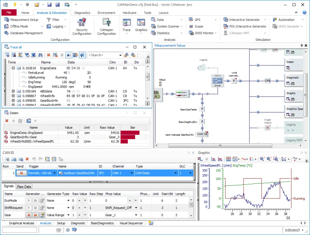
With CANalyzer you can do Analysis, Diagnostics, Logging, and Simulation.
CANalyzer comes with various options with a Basic version supporting CAN, LIN, Ethernet, FlexRay, and MOST and higher versions supporting J1939, CANopen, etc.
CANLab
CANLab is a network analysis tool used for the analysis of CAN bus network analysis.
Supports CAN FD, J1939, and LIN. Can be used with a variety of CAN interfaces.
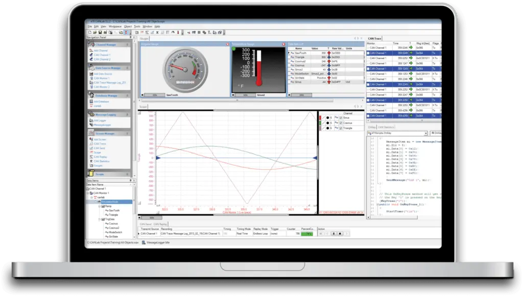
CANLab can be used to view and analyze network activities, record the data, replay the data, send and receive the CAN messages, simulate.
It also supports scripting using C# language. CANLab is mainly used as an automotive CAN bus analyzer tool.
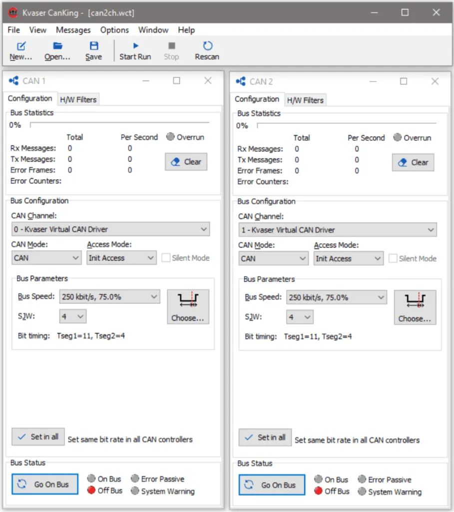
CanKing
CanKing is a CAN bus analyzer tool free of cost. Supports CAN FD. Suited for development work. You can send and receive CAN messages, log the data, filter messages, virtual CAN channels.
CANtrace
CANtrace is an easy-to-use CAN analyzer, that lets you trace, decode and plot CAN messages and signals in real-time, or log everything for post-processing.
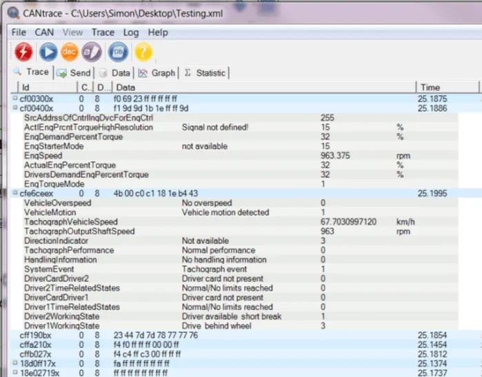
It works with variety of hardware. It supports J1939 and CANopen.
Raptor-CAN
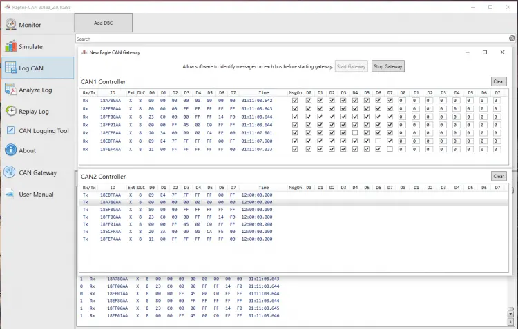
Raptor-CAN offers a simple, low-cost, and easy-to-use solution for practically any CAN bus monitoring & debugging needs.
It can monitor, log, or send data to the CAN bus. It allows resending the recorded data.
CanEasy
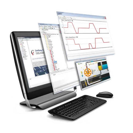
CanEasy is a Windows-based development tool used for simulation, analysis of the CAN bus network.
Supports UDS and XCP/CCP diagnostic functions. It works with industry-standard CAN interfaces.
Due to the automatically generated panels, the high level of automation and programmability, CanEasy can be used very quickly and flexibly.
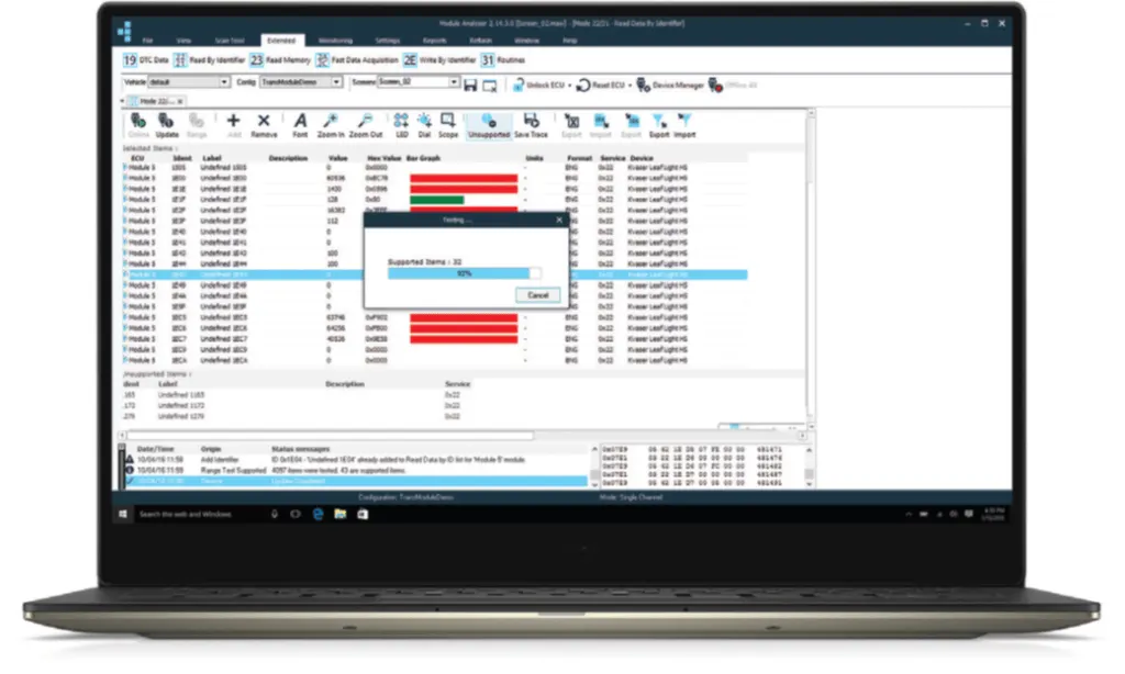
Module Analyser
Module Analyser used to acquire, view and monitor CAN, LIN, and FlexRay BUS traffic.
It can be used to monitor the CAN network bus integrity and for troubleshooting. Also used for CAN and LIN node simulation.
It supports OBD, UDS, J1939. Module Analyser has data logging capability.
EASY CAN
EASY CAN is a CAN network interface and analysis tool for Kvaser CAN interfaces. It is used to view, send, and record CAN data.
EASY CAN offers powerful basic functions for beginners as well as extensive detailed functions for experienced users. It also includes advanced analysis tools.
EASY CAN is not linked to your PC, your Kvaser CAN interface will be your dongle.
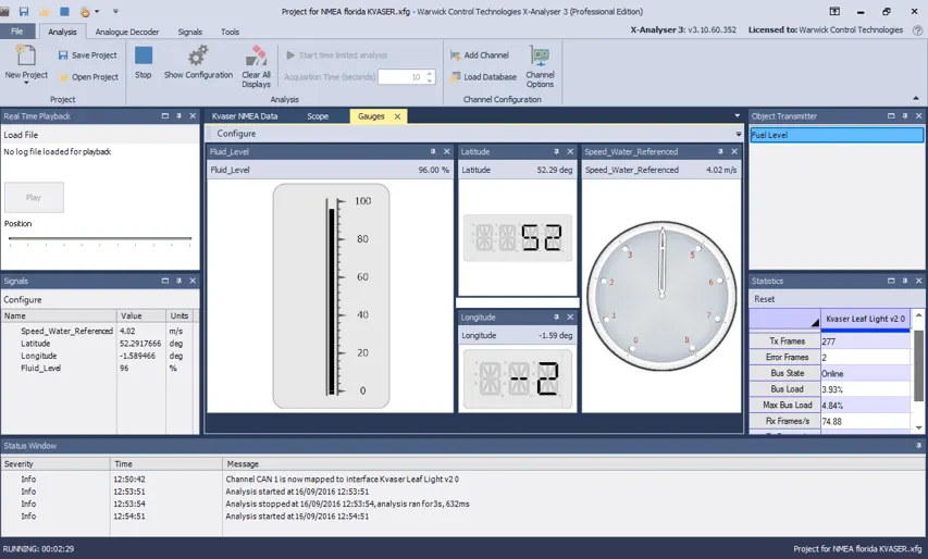
X-Analyser
The X-Analyser is a powerful, low-cost Windows-based tool that uses Kvaser or Vector interfaces to test your CAN/CANopen/J1939/NMEA2000/DeviceNet and LIN bus systems.
It can also be used for OBD scan tool functions over the CAN bus. Simulate CAN, CAN FD & LIN Devices or Network.
Build messages for transmission on a CAN, CAN FD, or LIN bus from a .DBC or .LDF file.
Conclusion
There you have it: 9 BEST CAN analyzer tools.
Now I’d like to hear from you:
Are there any quality CAN analyzer tools here that I missed?
Or maybe you have a question about one of the tools I listed.
Either way, leave a quick comment below right now.