Project 2
PLEASE FIND THE ATTACHED FILE ALSO
# Project 2
##Implementation of Clustering and then prediction the class of car from “Car dataset”.
import pandas as pd
import numpy as np
import matplotlib.pyplot as plt
import seaborn as sns
from scipy.sparse import hstack
from sklearn.preprocessing import StandardScaler, OneHotEncoder
from sklearn.model_selection import train_test_split
from sklearn.cluster import KMeans, AgglomerativeClustering
from sklearn.manifold import TSNE
from sklearn.metrics import mean_squared_error
import warnings
warnings.filterwarnings("ignore")
df = pd.read_csv("clean_auto.csv")
print(df)
symboling normalized-losses make aspiration num-of-doors \
0 3 122 alfa-romero std two
1 3 122 alfa-romero std two
2 1 122 alfa-romero std two
3 2 164 audi std four
4 2 164 audi std four
.. ... ... ... ... ...
196 -1 95 volvo std four
197 -1 95 volvo turbo four
198 -1 95 volvo std four
199 -1 95 volvo turbo four
200 -1 95 volvo turbo four
body-style drive-wheels engine-location wheel-base length ... \
0 convertible rwd front 88.6 0.811148 ...
1 convertible rwd front 88.6 0.811148 ...
2 hatchback rwd front 94.5 0.822681 ...
3 sedan fwd front 99.8 0.848630 ...
4 sedan 4wd front 99.4 0.848630 ...
.. ... ... ... ... ... ...
196 sedan rwd front 109.1 0.907256 ...
197 sedan rwd front 109.1 0.907256 ...
198 sedan rwd front 109.1 0.907256 ...
199 sedan rwd front 109.1 0.907256 ...
200 sedan rwd front 109.1 0.907256 ...
compression-ratio horsepower peak-rpm city-mpg highway-mpg price \
0 9.0 111.0 5000.0 21 27 13495.0
1 9.0 111.0 5000.0 21 27 16500.0
2 9.0 154.0 5000.0 19 26 16500.0
3 10.0 102.0 5500.0 24 30 13950.0
4 8.0 115.0 5500.0 18 22 17450.0
.. ... ... ... ... ... ...
196 9.5 114.0 5400.0 23 28 16845.0
197 8.7 160.0 5300.0 19 25 19045.0
198 8.8 134.0 5500.0 18 23 21485.0
199 23.0 106.0 4800.0 26 27 22470.0
200 9.5 114.0 5400.0 19 25 22625.0
city-L/100km horsepower-binned diesel gas
0 11.190476 Medium 0 1
1 11.190476 Medium 0 1
2 12.368421 Medium 0 1
3 9.791667 Medium 0 1
4 13.055556 Medium 0 1
.. ... ... ... ...
196 10.217391 Medium 0 1
197 12.368421 High 0 1
198 13.055556 Medium 0 1
199 9.038462 Medium 1 0
200 12.368421 Medium 0 1
[201 rows x 29 columns]
df.columns
df.columns
Index(['symboling', 'normalized-losses', 'make', 'aspiration', 'num-of-doors',
'body-style', 'drive-wheels', 'engine-location', 'wheel-base', 'length',
'width', 'height', 'curb-weight', 'engine-type', 'num-of-cylinders',
'engine-size', 'fuel-system', 'bore', 'stroke', 'compression-ratio',
'horsepower', 'peak-rpm', 'city-mpg', 'highway-mpg', 'price',
'city-L/100km', 'horsepower-binned', 'diesel', 'gas']
df.info()
<class 'pandas.core.frame.DataFrame'>
RangeIndex: 201 entries, 0 to 200
Data columns (total 29 columns):
# Column Non-Null Count Dtype
--- ------ -------------- -----
0 symboling 201 non-null int64
1 normalized-losses 201 non-null int64
2 make 201 non-null object
3 aspiration 201 non-null object
4 num-of-doors 201 non-null object
5 body-style 201 non-null object
6 drive-wheels 201 non-null object
7 engine-location 201 non-null object
8 wheel-base 201 non-null float64
9 length 201 non-null float64
10 width 201 non-null float64
11 height 201 non-null float64
12 curb-weight 201 non-null int64
13 engine-type 201 non-null object
14 num-of-cylinders 201 non-null object
15 engine-size 201 non-null int64
16 fuel-system 201 non-null object
17 bore 201 non-null float64
18 stroke 197 non-null float64
19 compression-ratio 201 non-null float64
20 horsepower 201 non-null float64
21 peak-rpm 201 non-null float64
22 city-mpg 201 non-null int64
23 highway-mpg 201 non-null int64
24 price 201 non-null float64
25 city-L/100km 201 non-null float64
26 horsepower-binned 200 non-null object
27 diesel 201 non-null int64
28 gas 201 non-null int64
df.describe()
symboling normalized-losses wheel-base length width height curb-weight engine-size bore stroke compression-ratio horsepower peak-rpm city-mpg highway-mpg price city-L/100km diesel gas
count 201.000000 201.00000 201.000000 201.000000 201.000000 201.000000 201.000000 201.000000 201.000000 197.000000 201.000000 201.000000 201.000000 201.000000 201.000000 201.000000 201.000000 201.000000 201.000000
mean 0.840796 122.00000 98.797015 0.837102 0.915126 53.766667 2555.666667 126.875622 3.330692 3.256904 10.164279 103.405534 5117.665368 25.179104 30.686567 13207.129353 9.944145 0.099502 0.900498
std 1.254802 31.99625 6.066366 0.059213 0.029187 2.447822 517.296727 41.546834 0.268072 0.319256 4.004965 37.365700 478.113805 6.423220 6.815150 7947.066342 2.534599 0.300083 0.300083
min -2.000000 65.00000 86.600000 0.678039 0.837500 47.800000 1488.000000 61.000000 2.540000 2.070000 7.000000 48.000000 4150.000000 13.000000 16.000000 5118.000000 4.795918 0.000000 0.000000
25% 0.000000 101.00000 94.500000 0.801538 0.890278 52.000000 2169.000000 98.000000 3.150000 3.110000 8.600000 70.000000 4800.000000 19.000000 25.000000 7775.000000 7.833333 0.000000 1.000000
50% 1.000000 122.00000 97.000000 0.832292 0.909722 54.100000 2414.000000 120.000000 3.310000 3.290000 9.000000 95.000000 5125.369458 24.000000 30.000000 10295.000000 9.791667 0.000000 1.000000
75% 2.000000 137.00000 102.400000 0.881788 0.925000 55.500000 2926.000000 141.000000 3.580000 3.410000 9.400000 116.000000 5500.000000 30.000000 34.000000 16500.000000 12.368421 0.000000 1.000000
max 3.000000 256.00000 120.900000 1.000000 1.000000 59.800000 4066.000000 326.000000 3.940000 4.170000 23.000000 262.000000 6600.000000 49.000000 54.000000 45400.000000 18.076923 1.000000 1.000000
df.info()
<class 'pandas.core.frame.DataFrame'>
RangeIndex: 201 entries, 0 to 200
Data columns (total 29 columns):
# Column Non-Null Count Dtype
--- ------ -------------- -----
0 symboling 201 non-null int64
1 normalized-losses 201 non-null int64
2 make 201 non-null object
3 aspiration 201 non-null object
4 num-of-doors 201 non-null object
5 body-style 201 non-null object
6 drive-wheels 201 non-null object
7 engine-location 201 non-null object
8 wheel-base 201 non-null float64
9 length 201 non-null float64
10 width 201 non-null float64
11 height 201 non-null float64
12 curb-weight 201 non-null int64
13 engine-type 201 non-null object
14 num-of-cylinders 201 non-null object
15 engine-size 201 non-null int64
16 fuel-system 201 non-null object
17 bore 201 non-null float64
18 stroke 197 non-null float64
19 compression-ratio 201 non-null float64
20 horsepower 201 non-null float64
21 peak-rpm 201 non-null float64
22 city-mpg 201 non-null int64
23 highway-mpg 201 non-null int64
24 price 201 non-null float64
25 city-L/100km 201 non-null float64
26 horsepower-binned 200 non-null object
27 diesel 201 non-null int64
28 gas 201 non-null int64
df
symboling normalized-losses make aspiration num-of-doors body-style drive-wheels engine-location wheel-base length ... compression-ratio horsepower
0 3 122 alfa-romero std two convertible rwd front 88.6 0.811148 ... 9.0 111.0 5000.0 21 27 13495.0 11.190476 Medium 0 1
1 3 122 alfa-romero std two convertible rwd front 88.6 0.811148 ... 9.0 111.0 5000.0 21 27 16500.0 11.190476 Medium 0 1
2 1 122 alfa-romero std two hatchback rwd front 94.5 0.822681 ... 9.0 154.0 5000.0 19 26 16500.0 12.368421 Medium 0 1
3 2 164 audi std four sedan fwd front 99.8 0.848630 ... 10.0 102.0 5500.0 24 30 13950.0 9.791667 Medium 0 1
4 2 164 audi std four sedan 4wd front 99.4 0.848630 ... 8.0 115.0 5500.0 18 22 17450.0 13.055556 Medium 0 1
... ... ... ... ... ... ... ... ... ... ... ... ... ... ... ... ... ... ... ... ... ...
196 -1 95 volvo std four sedan rwd front 109.1 0.907256 ... 9.5 114.0 5400.0 23 28 16845.0 10.217391 Medium 0 1
197 -1 95 volvo turbo four sedan rwd front 109.1 0.907256 ... 8.7 160.0 5300.0 19 25 19045.0 12.368421 High 0 1
198 -1 95 volvo std four sedan rwd front 109.1 0.907256 ... 8.8 134.0 5500.0 18 23 21485.0 13.055556 Medium 0 1
199 -1 95 volvo turbo four sedan rwd front 109.1 0.907256 ... 23.0 106.0 4800.0 26 27 22470.0 9.038462 Medium 1 0
200 -1 95 volvo turbo four sedan rwd front 109.1 0.907256 ... 9.5 114.0 5400.0 19 25 22625.0 12.368421 Medium 0 1
201 rows × 29 columns
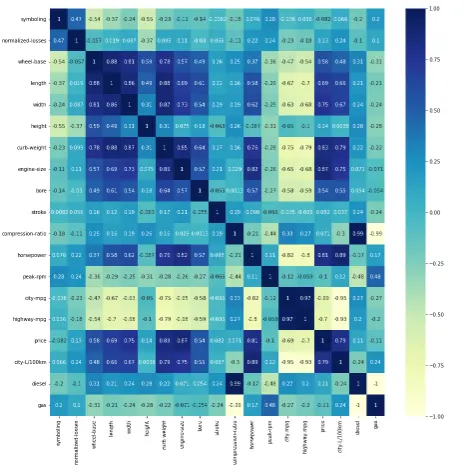
plt.subplots(figsize = ([15,15]))
sns.heatmap(df.corr(),cmap = 'YlGnBu',annot = True)
new_df = df[['make','city-mpg','price']]
new_df
make city-mpg price
0 alfa-romero 21 13495.0
1 alfa-romero 21 16500.0
2 alfa-romero 19 16500.0
3 audi 24 13950.0
4 audi 18 17450.0
... ... ... ...
196 volvo 23 16845.0
197 volvo 19 19045.0
198 volvo 18 21485.0
199 volvo 26 22470.0
200 volvo 19 22625.0
201 rows × 3 columns
X = new_df.iloc[:,[1,2]]
X
city-mpg price
0 21 13495.0
1 21 16500.0
2 19 16500.0
3 24 13950.0
4 18 17450.0
... ... ...
196 23 16845.0
197 19 19045.0
198 18 21485.0
199 26 22470.0
200 19 22625.0
201 rows × 2 columns
Y = new_df.iloc[:,[0]]
Y
make
0 alfa-romero
1 alfa-romero
2 alfa-romero
3 audi
4 audi
... ...
196 volvo
197 volvo
198 volvo
199 volvo
200 volvo
201 rows × 1 columns
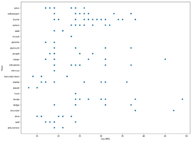
plt.figure(figsize = (15,12))
plt.scatter(X['city-mpg'],Y['make'])
plt.xlabel('City MPG')
plt.ylabel('Make')
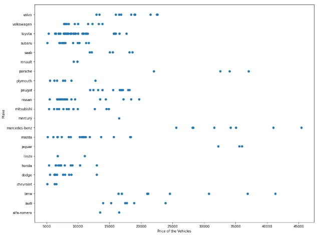
plt.figure(figsize = (15,12))
plt.scatter(X['price'],Y['make'])
plt.xlabel('Price of the Vehicles')
plt.ylabel('Make')
scaler = StandardScaler()
scaler.fit(X)
scaled_X = pd.DataFrame(scaler.transform(X),columns = X.columns)
scaled_X
city-mpg price
0 -0.652249 0.036314
1 -0.652249 0.415385
2 -0.964397 0.415385
3 -0.184027 0.093711
4 -1.120471 0.535224
... ... ...
196 -0.340101 0.458906
197 -0.964397 0.736429
198 -1.120471 1.044227
199 0.128120 1.168481
200 -0.964397 1.188034
201 rows × 2 columns
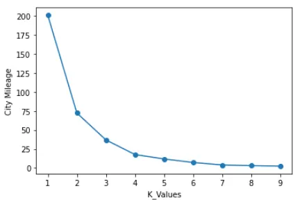
k_rng = range(1,10)
sse1 = []
for k1 in k_rng:
km1 = KMeans(n_clusters = k1)
km1.fit(scaled_X[['city-mpg']])
sse1.append(km1.inertia_)
plt.xlabel('K_Values')
plt.ylabel('City Mileage')
plt.plot(k_rng,sse1,marker = 'o')
km1 = KMeans(n_clusters = 3)
km1.fit(scaled_X[['city-mpg']])
y_predict = km1.predict(scaled_X[['city-mpg']])
MC_df = pd.concat([scaled_X['city-mpg'],Y['make']],axis = 1)
MC_df['Cluster(M vs C)'] = y_predict
MC_df
city-mpg make Cluster(M vs C)
0 -0.652249 alfa-romero 0
1 -0.652249 alfa-romero 0
2 -0.964397 alfa-romero 0
3 -0.184027 audi 2
4 -1.120471 audi 0
... ... ... ...
196 -0.340101 volvo 2
197 -0.964397 volvo 0
198 -1.120471 volvo 0
199 0.128120 volvo 2
200 -0.964397 volvo 0
201 rows × 3 columns
MC_df1 = MC_df[MC_df['Cluster(M vs C)'] == 0]
MC_df2 = MC_df[MC_df['Cluster(M vs C)'] == 1]
MC_df3 = MC_df[MC_df['Cluster(M vs C)'] == 2]
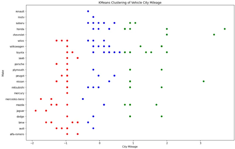
plt.subplots(figsize = ([15,10]))
plt.scatter(MC_df1['city-mpg'],MC_df1['make'],color = 'red')
plt.scatter(MC_df2['city-mpg'],MC_df2['make'],color = 'green')
plt.scatter(MC_df3['city-mpg'],MC_df3['make'],color = 'blue')
plt.title('KMeans Clustering of Vehicle City Mileage')
plt.xlabel('City Mileage')
plt.ylabel('Make')
 km2 = KMeans(n_clusters = 3)
km2.fit(scaled_X[['price']])
y_predict = km1.predict(scaled_X[['price']])
MP_df = pd.concat([scaled_X['price'],Y['make']],axis = 1)
MP_df['Cluster(M vs P)'] = y_predict
MP_df
price make Cluster(M vs P)
0 0.036314 alfa-romero 2
1 0.415385 alfa-romero 2
2 0.415385 alfa-romero 2
3 0.093711 audi 2
4 0.535224 audi 2
... ... ... ...
196 0.458906 volvo 2
197 0.736429 volvo 1
198 1.044227 volvo 1
199 1.168481 volvo 1
200 1.188034 volvo 1
201 rows × 3 columns
MP_df1 = MP_df[MP_df['Cluster(M vs P)'] == 0]
MP_df2 = MP_df[MP_df['Cluster(M vs P)'] == 1]
MP_df3 = MP_df[MP_df['Cluster(M vs P)'] == 2]
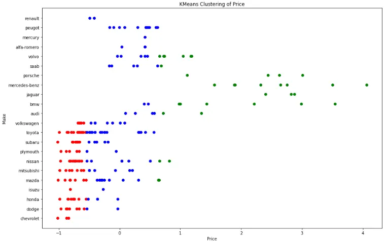
plt.subplots(figsize = ([15,10]))
plt.scatter(MP_df1['price'],MP_df1['make'],color = 'red')
plt.scatter(MP_df2['price'],MP_df2['make'],color = 'green')
plt.scatter(MP_df3['price'],MP_df3['make'],color = 'blue')
plt.title('KMeans Clustering of Price')
plt.xlabel('Price')
plt.ylabel('Make')
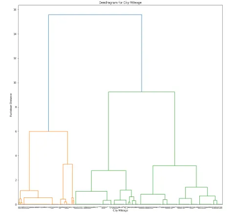
 plt.figure(figsize = (15,15))
import scipy.cluster.hierarchy as sch
dendrograms = sch.dendrogram(sch.linkage(scaled_X[['city-mpg']],method = 'ward'))
plt.title('Dendrogram for City Mileage')
plt.xlabel('City Mileage')
plt.ylabel('Euclidean Distance')
plt.figure(figsize = (15,15))
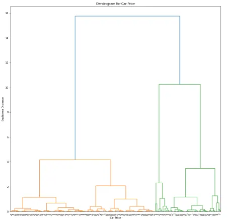
dendrograms = sch.dendrogram(sch.linkage(scaled_X[['price']],method = 'ward'))
plt.title('Dendrogram for Car Price')
plt.xlabel('Car Price')
plt.ylabel('Euclidean Distance')
hc = AgglomerativeClustering(n_clusters = 3,affinity = 'euclidean',linkage = 'ward')
hc_predict_mpg = hc.fit_predict(scaled_X[['city-mpg']])
mpg = pd.concat([scaled_X['city-mpg'],Y['make']],axis = 1)
mpg['Clusters'] = hc_predict_mpg
mpg
city-mpg make Clusters
0 -0.652249 alfa-romero 2
1 -0.652249 alfa-romero 2
2 -0.964397 alfa-romero 2
3 -0.184027 audi 1
4 -1.120471 audi 2
... ... ... ...
196 -0.340101 volvo 1
197 -0.964397 volvo 2
198 -1.120471 volvo 2
199 0.128120 volvo 1
200 -0.964397 volvo 2
201 rows × 3 columns
hc = AgglomerativeClustering(n_clusters = 3,affinity = 'euclidean',linkage = 'ward')
hc_predict_price = hc.fit_predict(scaled_X[['price']])
price = pd.concat([scaled_X['price'],Y['make']],axis = 1)
price['Clusters'] = hc_predict_price
price
price make Clusters
0 0.036314 alfa-romero 0
1 0.415385 alfa-romero 1
2 0.415385 alfa-romero 1
3 0.093711 audi 0
4 0.535224 audi 1
... ... ... ...
196 0.458906 volvo 1
197 0.736429 volvo 1
198 1.044227 volvo 1
199 1.168481 volvo 1
200 1.188034 volvo 1
201 rows × 3 columns
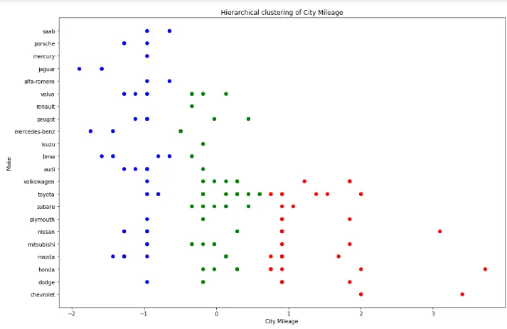
mpg1 = mpg[mpg['Clusters'] == 0]
mpg2 = mpg[mpg['Clusters'] == 1]
mpg3 = mpg[mpg['Clusters'] == 2]
plt.subplots(figsize = ([15,10]))
plt.scatter(mpg1['city-mpg'],mpg1['make'],color = 'red')
plt.scatter(mpg2['city-mpg'],mpg2['make'],color = 'green')
plt.scatter(mpg3['city-mpg'],mpg3['make'],color = 'blue')
plt.title('Hierarchical clustering of City Mileage')
plt.xlabel('City Mileage')
plt.ylabel('Make')
price1 = price[price['Clusters'] == 0]
price2 = price[price['Clusters'] == 1]
price3 = price[price['Clusters'] == 2]
plt.subplots(figsize = ([15,10]))
plt.scatter(price1['price'],price1['make'],color = 'red')
plt.scatter(price2['price'],price2['make'],color = 'green')
plt.scatter(price3['price'],price3['make'],color = 'blue')
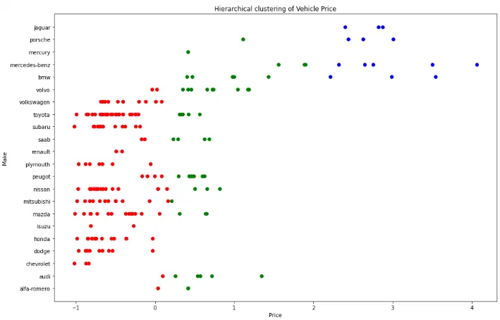
plt.title('Hierarchical clustering of Vehicle Price')
plt.xlabel('Price')
plt.ylabel('Make')