Project 2

in the model in fig 1.2, the input drive cycle data taken is a drive cycle source for 2474 sec. This drive cycle data is then fed into the Longitudinal driver block. It takes reference velocity and velocity feedback. Also, a grade can also be entered to simulate the hill climb. Here, we are considering no hill climb condition, so, the value is taken as zero. This block outputs acceleration and deceleration commands into the motor controller. In the controller subsystem, the commands from the driver are entered as input data. The commands from the acceleration port are given to the PWM port of the H-bridge, through a controlled PWM Voltage source. The deceleration commands are given into the BRK port of the H-bridge. All the references are grounded. The positive and negative terminals are connected to the DC motor. Different parameters that are used for the simulation are shown below.

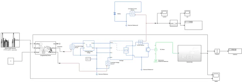
Fig 1.2

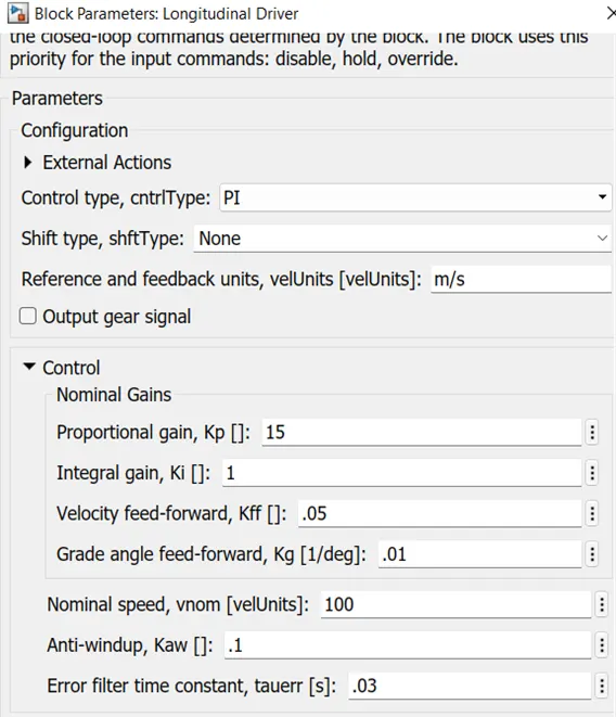
Fig 1.3

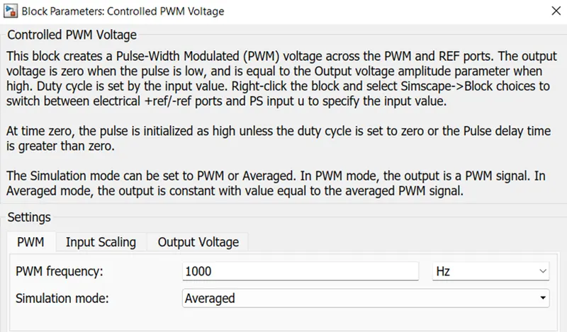
Fig 1.4

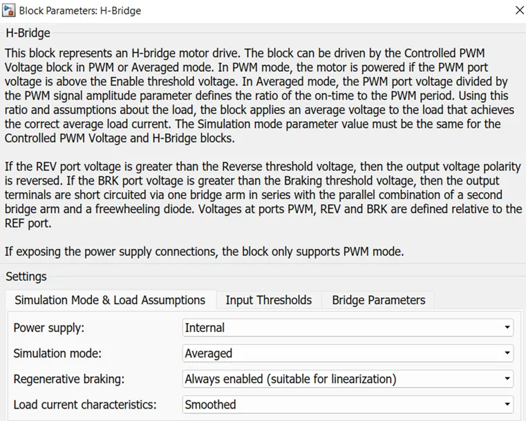
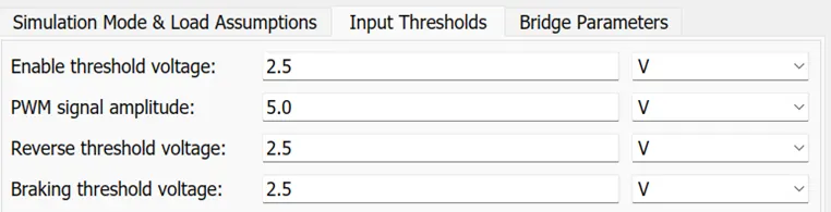
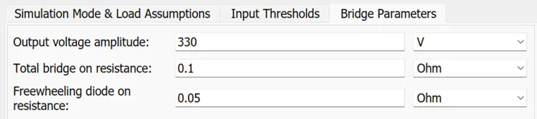
Fig 1.5

The positive of the H-bridge is also connected to a battery source through a current sensor. Moving onto the DC Motor, the motor controlled fed the voltage through a controlled battery source as shown above into the DC Motor. In the motor, the shaft output is connected to the gear box and the motor casing is connected to a mechanical rotational reference. Battery and DC Motor parameters are shown below;

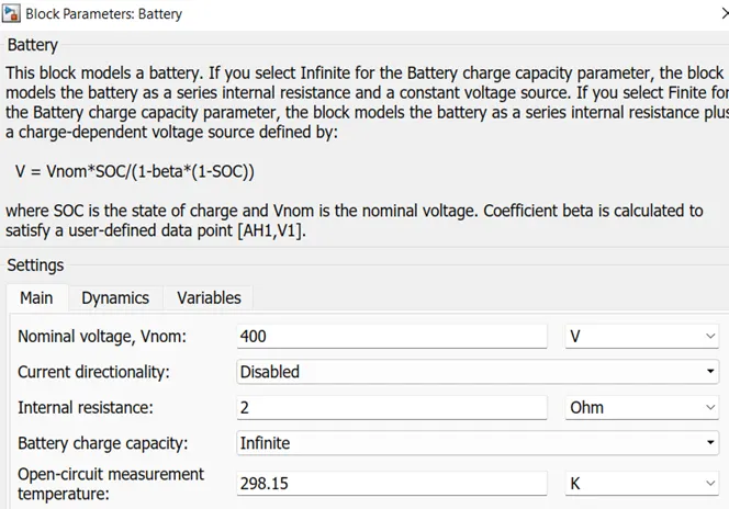
Fig 1.6

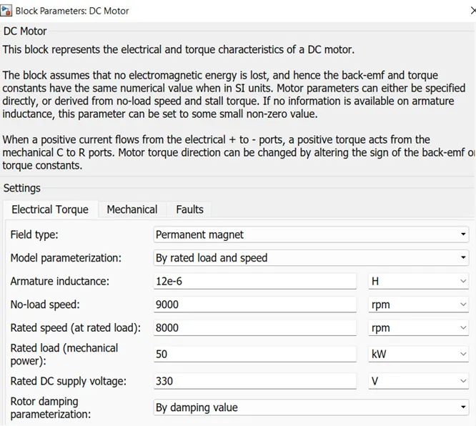
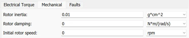
Fig 1.7

The R-port of the DC motor is connected to a subsystem titled ‘Vehicle body’. The internal diagram of the subsystem is given below.

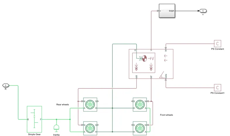
Fig 1.8

Input of the subsystem is a PMC port titled ‘R’ which is connected to a simple gear. The parameters of the simple gear taken are given below.

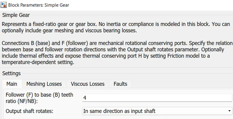
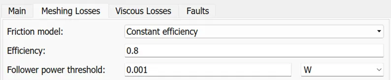
Fig 1.9

Inertia block is also taken into consideration. The simple gear is connected to the 4 tire blocks. Since, this is a rear wheel drive, the motor shaft is connected to the rear axle of the car. The parameters taken in the tire blocks are shown below.

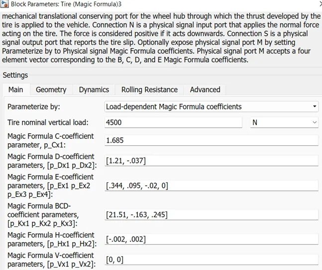
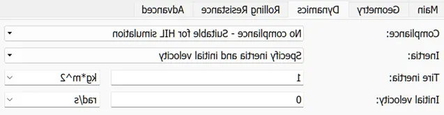
Fig 1.10

All the wheel hubs are connected to the hub of the vehicle body block set. N port is for the normal force acting on the wheel. So, they are connected to the NR and NF for Rear and Front respectively. And the V-port of the vehicle body block set is connected to an output PMC port of the subsystem titled as ‘V’. The vehicle body block parameters given are;

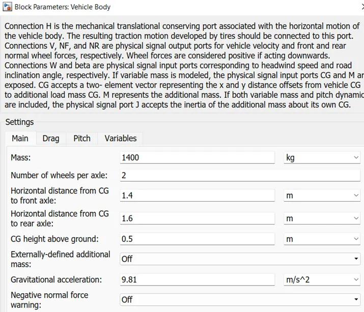
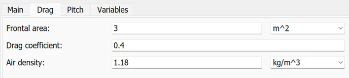
Fig 1.11

The output of the subsystem is connected to an integrator block through a PS-Simulink converter and then to a display block to calculating the total distance travelled by the electrical vechicle. A scope is taken from the VelFdbk port of the longitudinal driver and the output of the subsystem for determining the variation of speed with time. Another subsystem titled ‘SOC Estimate’ is taken from the negative terminal of the current sensor, along with a scope to determine the variation of current with time. The internal diagram of this subsystem is given below.

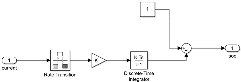
Fig 1.12

The input of the subsystem is a PMC port titled [A] which is connected to a rate transition block and then to a gain block with the value 1/(80*3600). It is then connected to a discrete-time integrator and given to an add block that adds the given signal with a constant block of value 1 and gives the result to an output PMC port titled SOC[0, 1]. Lastly, a scope and display blocks are taken from the output of this subsystem for calculating the SOC value and determining the variation of SOC with respect to time.

RESULTS

1. Speed vs Time plot

From the curves for the actual speed and the command speed, it is evident that the velocity feedback (actual speed) very closely traces the input velocity (command speed). Only, at instants where the drive cycle velocity is declining abruptly, the velocity feedback comes to zero at a slower rate than the former, because practically the vehicle will come to a halt after in some time. So, a slow negative acceleration is shown.

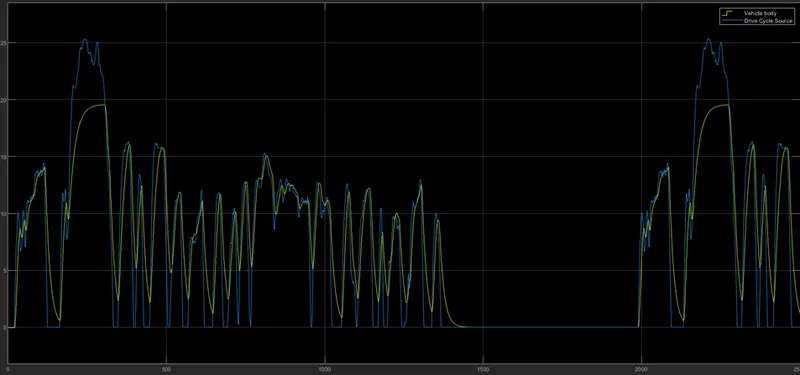
Fig 1.13

2. Current vs Time plot

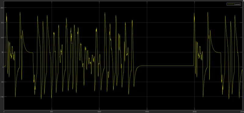
Fig 1.14

Here, the current curve fluctuates in the positive and negative halves in between 168.3 A and -110.25 A from 0 to 1500 sec. Then, the value becomes zero in between 1500 to 2000 sec, as it follows the drive cycle which is similarly zero during this time interval. Then, for the rest of the time it continues to fluctuate in the negative and positive halves as before.

3. SOC vs Time plot

The SOC of the battery goes from 100% to around 79.21%, where there is a decrease in the SOC by about 20.8%. In some intervals this value increases, that is representing the regenerative braking. During this period the motor is acting as a generator and is feeding the charge back into the battery, thus charging the battery.v