Project 2
Aim:
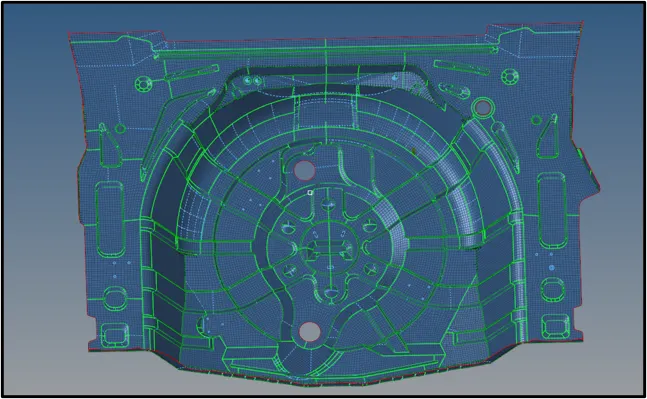
To check for the geometrical errors and to extract the midsurface of the given component and to complete the 2D meshing for the component considering the given quality criteria.
Abstract:
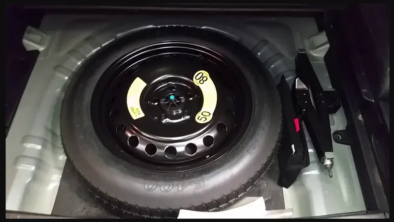
The floorpan is a large sheet metal stamping that often incorporates several smaller welded stampings to form the floor of a large vehicle and the position of its external and structural panels. In the case of monocoque designs, the floorpan is the most important metal part establishing the chassis, body, and thus the car's size. It serves as the foundation of most of the structural and mechanical components of a unibody automobile to which the powertrain, suspension system, and other parts are attached. The term is also applied to the smaller stamped panels that form the floors inside a vehicle as well as the bottom of the trunk.
A structural shear panel for forming a floor panel for support by a vehicle frame is formed by a composite of top and bottom sheets and a core with a vacuum infused resin. The core is formed of top and bottom layers each formed from a honeycomb panel defining an array of hexagonal tubular cells with walls which extend in the thickness direction filled with a foam material. A third layer is located between the first and second layers and is formed of a material such as foam, rubber or cork which is free from tubular cells in the thickness direction and free from rigid structural members in the thickness direction to reduce communication of sound through the panel.
Introduction To FEA :
What is FEA?
Finite element analysis (FEA) is a computerized method for predicting how a product reacts to real-world forces, vibration, heat, fluid flow, and other physical effects. Finite element analysis shows whether a product will break, wear out, or work the way it was designed.
It is necessary to use mathematics to comprehensively understand and quantify any physical phenomena such as structural or fluid behavior, thermal transport, wave propagation, the growth of biological cells, etc. Most of these processes are described using Partial Differential Equations (PDEs). However, for a computer to solve these PDEs, numerical techniques have been developed over the last few decades and one of the prominent ones, today, is the Finite Element Analysis.
Differential equations not only describe natural phenomena but also physical phenomena encountered in engineering mechanics. These partial differential equations (PDEs) are complicated equations that need to be solved in order to compute relevant quantities of a structure (like stresses (ϵ), strains (ϵ), etc.) in order to estimate the structural behavior under a given load. It is important to know that FEA only gives an approximate solution to the problem and is a numerical approach to get the real result of these partial differential equations. Simplified, FEA is a numerical method used for the prediction of how a part or assembly behaves under given conditions. It is used as the basis for modern simulation software and helps engineers to find weak spots, areas of tension, etc. in their designs. The results of a simulation based on the FEA method are usually depicted via a color scale that shows, for example, the pressure distribution over the object.
Advantages of FEA :
- Enhanced design and early evaluation of critical design parameters.
- Virtual prototyping capability, meaning fewer physical prototypes are required and which are aligned to rapid prototyping.
- Efficient and less expensive design cycles.
- Increased productivity, and profit.
- De-risked design process.
- Reports can be produced as part of quality control and audit processes.
- Maximise performance through material selection and cost-efficiency.
- Reduced R&D and development costs.
- Certification or verification- The simulation data output is only as good as the input data. We have the engineering experience, expertise, and calibre to identify any potential anomalies. We will cross-check and carry out calculations to ensure the data output is correct.
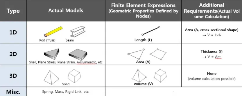
Types of Finite Elements:
- 1D Element
- 2D Element
- 3D Element
Meshing :
A mesh is a group of interconnected finite elements joined together at nodes that represents the shape of continuous geometry, including both the external surface and the interior volume. A mesh can also be thought of as the CAD model being “chopped up” into discrete pieces (finite elements) that are connected together. Because these elements are geometrically quite simple, the equations associated with each individual element are relatively simple, so that when the mesh is assembled into a matrix of equations, we can solve complex geometries by solving a large number of simple equations.
The first step for numerically solving a set of partial differential equations (PDEs) is the discretization of the equations and the discretization of the problem domain. As mentioned earlier, solving the entire problem domain at once is impossible whereas solving multiple small pieces of the problem domain is perfectly fine. The equations discretization process is related to methods such as the Finite Difference Method, Finite Volume Method (FVM) and Finite Element Method, whose purpose is to take equations in the continuous form and generate a system of algebraic difference equations. The domain discretization process generates a set of discrete cells and therefore points or nodes that cover the continuous problem domain.
A mesh is, by definition, a set of points and cells, when connected to form a network. This network can have many forms of geometry and topology, as will be discussed later. Often, meshes are also called grids, and that is generally related to the intrinsic organization of the mesh and/or when those meshes are related to Finite Differences problems.
Each cell or node of the mesh will hold a local solution of the equations, depending on whether the equations were discretized over the cells or nodes. The choice of discretization is a project decision.
In general, point discretization is used when the equations are approximated using the Finite Differences Method, where the PDEs are usually approximated by Taylor series expansions at each point’s neighbors. Sometimes the point discretization can be used together with the Finite Volume Method, however, cells are going to be implicitly used around points.
Mesh Types :
It’s common to classify mesh types as structured (curvilinear) or unstructured.
Structured Mesh :
Structured meshes, also commonly called grids, are meshes whose structure and formation allow for easy identification of neighboring cells and points. This property is derived from the fact that structured meshes are applied over analytical coordinates systems (rectangular, elliptical, spherical, etc.), forming a regular grid.From a programming point of view, the cells or points that form a structured mesh can be enumerated in such a way that neighboring queries can be made analytically upon the cells or points coordinates.
Unstructured Mesh :
Unstructured meshes are more general and can arbitrarily approximate any geometry shape. In contrast with structured meshes, where the coordinates and connectivities map into the elements of a matrix, unstructured meshes require special data structures, such as an adjacency matrix or list and the node coordinates list. The unstructured mesh node/cell numbering can be arbitrary and sparse since it does not require any analytical form of adjacency query. Complex geometries that would be impractical to generate a structured mesh within, can be discretized using unstructured meshing techniques. The flexible nature of unstructured meshes allows various cell types to be used and coexist in the same mesh, making it possible to have an even better geometry fitting and overall element quality.
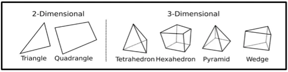
Cell types can be separated into 2-Dimensional cells and 3-Dimensional cells. Common 2-Dimensional cell types are the triangle and the quadrangle. Common 3-Dimensional cell types are the tetrahedron and the hexahedron but might also include the pyramid and wedge. These cell types form what is sometimes called the finite element zoo since these cell types are commonly used with Finite Element schemes. Finite Volume schemes are known for being more flexible in terms of the cell types being used, sometimes allowing for any kind of polygons and polyhedra.
Why Is 2D Meshing Carried Out On The Mid Surface?
- Accuracy of the end result can be way off with solid mesh elements
- The solid mesh approach, which needs 3 to 4 elements across the thickness, results in huge amount of elements and long running times
- Meshing nasty geometry with solid mesh elements needs preparation too
- Post processing of huge amount of solid element simulations takes ages
- The shell mesh approach creates a fast running accurate simulations
Approach for meshing :
- Spend sufficient time studying geometry.
- Check for symmetry.
- Geometry cleanup if necessary.
- Identify feasible splitting ways.
- Start meshing from critical areas.
- Split mesh strategy should be followed.
- Follow thumb rules during mesh.
- After meshing each area check connectivity between two meshes.
Given Quality criteria :
Target Element Length = 5mm
| S.N | Quality Criteria | Value |
| 1 | Aspect Ratio | 5 |
| 2 | Skewness | 45 |
| 3 | Warping | 15 |
| 4 | Taper | 0.5 |
| 5 | Min. Length | 2mm |
| 6 | Max. Length | 8mm |
| 7 | Min angle Quad | 45 |
| 8 | Max angle Quad | 135 |
| 9 | Min angle Tria | 20 |
| 10 | Max angle Tria | 120 |
| 10 | Tria % | 10 |
Procedure:
Step 1 :
Import the given model into hypermesh using the import command:
- Click on the import command on the tool bar.
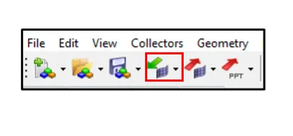
- Select the appropiate file type from the drop down menu (i.e STEP, IGES or HYPERMESH).
- Browse the file which is required to import.
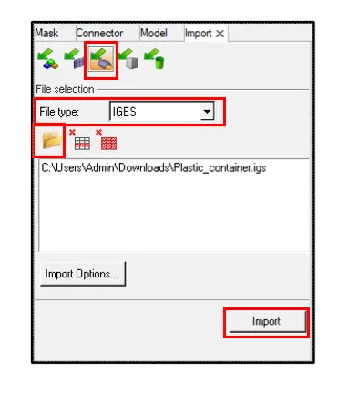
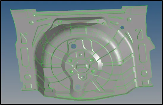
- Click import from the bottom and the required model will be displayed on the Hypermesh workbench.
Step 2:
Geometrical Cleanup and Topology of Parent model:
- Check for geomertrical errors in the parent model.
- Check for missing surfaces and free edges and fix it using the neccessary tools.
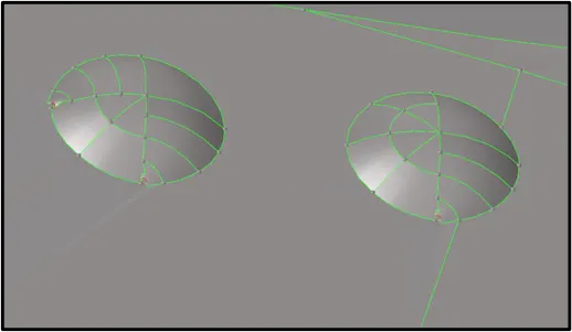
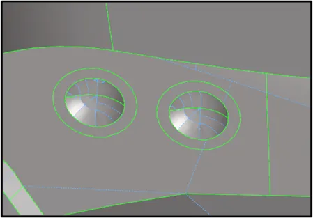
- Use the Quick Edit panel to split surfaces and washers, change the category (shared, free, and so on) of edges, create or delete surfaces and points, project points, and trim fillets.
- Check for the surfaces that might fail for minimum length and defeature if required using the defeature tool.
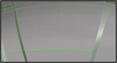
- Use the Edge Fillets subpanel to identify and remove edge fillets. Similar to surface fillets, edge fillets create smooth curves at the intersection of relatively perpendicular free edges. You can identify them based on the radius of the fillet arc, and then remove them.
- Use the line toggle option to toggle lines wherever required.
 .
. 
- Use the replace point option, to move points from their current locations to the locations of other points, effectively combining them.
Step 3 :
Extraction of midsurface :
Midsurface meshing is opted for components where the geometry thickness is small when compared with the span length of the components, so if you see most of the automotive structures are of sheet metal and plastics, where the length of the component is large when compared to the thickness, hence for this reason we opt for mid surface extraction and assign the thickness of the component to the elements through properties on components method.
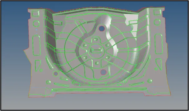
For this model, midsurface of the component can be extracted using auto mid command or the skin offset command
Use the Offset subpanel to offset a group of surfaces by a given distance along the normals of those surfaces. A negative offset value can be used to offset these surfaces in the opposite direction of the surface normal. The topology of the surface edges (free, shared edges, and so on) is maintained during the offset function. Some individual surfaces will be trimmed or extended to maintain the connectivity. This function moves the selected surfaces to the new location.If you want to save the original surfaces, the selected surfaces can be duplicated before the offset. You can review the normal direction of the surfaces by clicking vector normal or color normal. If the offset direction is incorrect, the reverse normal function can be used to reverse the normal of a selected surface. If there are elements associated to the offset surfaces, the element will not move along with surfaces. The association between the elements and their surfaces is broken.

Use the Midsurface panel to extract the midsurface representation of a solid part or to generate a finite element shell representation of a solid geometry. The Midsurface panel can be used to extract the midsurface of sheet metal stampings, molded plastic parts with ribs, and other parts that have thickness clearly smaller than width and length.
The midsurface subpanel consists of different tools to etxtract the midsuface of the component.
- Auto Midsurface Tool
Use the Auto Midsurface tool to extend and modify midsurfaces. - Interim Edit Tools
Use the Interim Edit tools to modify plates, base surfaces, and collapsed lines on the midsurface. - Final Edit Tools
Use the Final Edit tools repair surfaces, modify targets, and imprint surfaces after the midsurface has been extracted and you do not need to make further changes that require the midsurface to be re-extracted. - Review Thickness Tool
Use the Review Thickness tool to review the thickness of surfaces (including midsurfaces) and assign new fixed, uniform thicknesses to surfaces. - Sort Tool
Use the Sort tool to manually sort midsurfaces after extraction.

Step 4 :
Geometrical Cleanup and Topology of Midsurface :
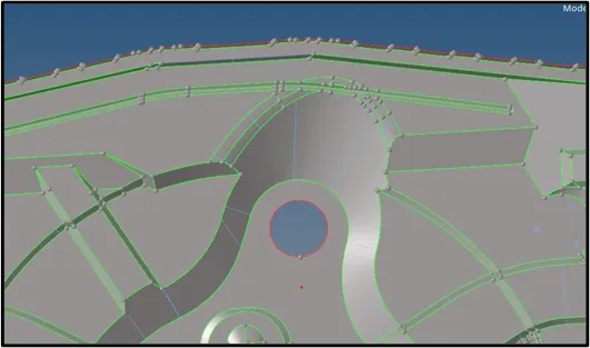
- Check for geomertrical errors in the midsurface.
- Check for missing surfaces and free edges and fix it using the neccessary tools.
- Use the Quick Edit panel to split surfaces and washers, change the category (shared, free, and so on) of edges, create or delete surfaces and points, project points, and trim fillets.
- Check for the surfaces that might fail for minimum length and defeature if required using the defeature tool.
- Use the Edge Fillets subpanel to identify and remove edge fillets. Similar to surface fillets, edge fillets create smooth curves at the intersection of relatively perpendicular free edges. You can identify them based on the radius of the fillet arc, and then remove them.
- Use the line toggle option to toggle lines wherever required.
- Use the replace point option, to move points from their current locations to the locations of other points, effectively combining them.
Step 5 :
Meshing the component :
Meshing is an integral part of the engineering simulation process where complex geometries are divided into simple elements that can be used as discrete local approximations of the larger domain. The mesh influences the accuracy, convergence and speed of the simulation.
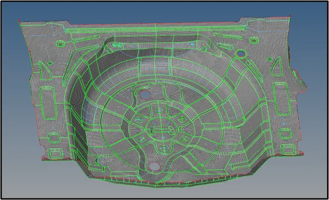
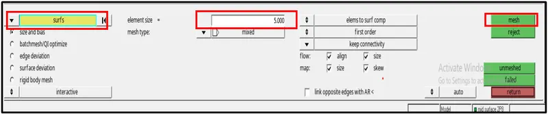
- Use the Automesh option to generate a mesh of plate elements using surface geometry or existing shell elements to define the mesh area.
- Set the options in the panel in any order that you feel comfortable using. Moving from subpanel to subpanel will not cause you to lose work. When you are finished making all your selections, click mesh to start the meshing process.
- Set the panel mode by selecting the appropriate subpanel.
- Select the meshing method by setting the entity selector to surfs or elems.
- Make the required element criteria settings.
- Set any algorithm options.
- Select the area to be meshed using the entity selector and any extended selection methods.
Step 6:
Check for quality errors :
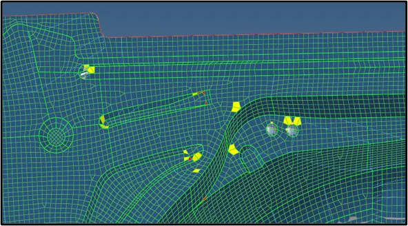
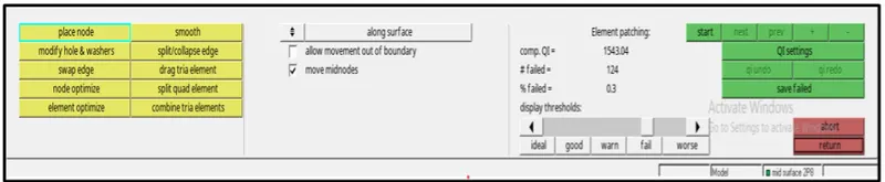
Use the Check Elems panel to verify the basic quality of your elements, as well as the geometric qualities of those elements.Each subpanel displays quality checks of a specific type, depending on dimensionality, time steps, and so forth. Each check is listed on a green command button; clicking the button performs a check and the results are summarized in the status bar.Criteria that you edit will be preserved even if you navigate to a different subpanel and then back again. However, criteria on different subpanels do not relate to each other, so changing the length requirement on the 1-d subpanel does not change the length requirement on the 2-d subpanel.Different checks are supplied to review the quality measurements of different types of elements. For example, if you have created a quad, it is possible that the quad has some degree of warpage. You can use the warpage function to check the element for warpage and to specify the maximum allowable warpage for that element.Another check available is for rigid loops. Use rigid loops to determine if a group of 1D rigid elements forms a loop. After it checks for instances where this has occurred, it highlights the elements that failed the test.
Criteria settings are stored and retrieved using a criteria file. You can save the results from the Quality Index (QI) panel to a summary file.
Step 7:
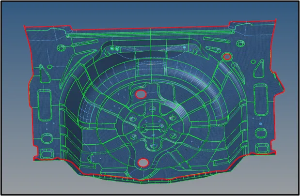
Check for Free edges :
Free edges are defined as a pair of nodes identifying an element edge that are not shared with another element. Free edges are normally found around the outer perimeter of a part or around openings within the part. Free edges found in your model are displayed as red plot elements in their own component called ^edges.

Step 8:
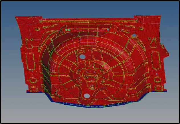
Check for Normals :
Use the Normals panel to display and reverse the normals of elements or surfaces. The orientation of element normals can also be adjusted. The normal of an element is determined by following the order of nodes of the element using the right-hand rule.For the Abaqus solver interface this panel can be used to adjust or reverse the stacking direction of continuum shells.Normals can be reviewed showing a vector or by colors. A vector shows in positive normal direction, while the color mode shows the positive side of a shell or surface in red and the negative side in blue.
Use the Elements subpanel to display and reverse the normals of elements. Select elements indirectly by components or directly by elements, or elect to have all of the displayed 2D elements selected automatically. Click display to review the current normal orientation of the selected elements. Optionally, click reverse to flip the normals to the opposite side (reverse the normals).You can also use the Elements subpanel to adjust element normals. Select elements to adjust, then select an orientation method which determines how element normals are adjusted. When you are finished, click adjust. Optionally, select display adjusted only to only display the elements which have been adjusted in this operation. All elements selected for adjusting must be in a continuous mesh for this operation.On review, normals are displayed with vectors by default. Alternatively, you can choose to display normals in color mode by switching the toggle from vector display normals to color display normals. Normals pointing in the wrong direction can be spotted easier in bigger meshes when using the color display mode. Red indicates the positive normal direction and blue indicates the opposite side of the element.In vector mode, specify the size of normals in the size field. If this value is zero, the normal is sized based on the smallest side of the element. If a value other than zero is specified for size, the normal is drawn based on the length specified in model units.

Step 9:
Assigning Thickness to elements :
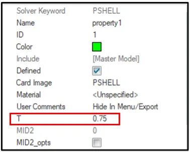
- After meshing, thickness needs to be assigned to the elements
- Create a new property and assign the thickness value as per the parent model.
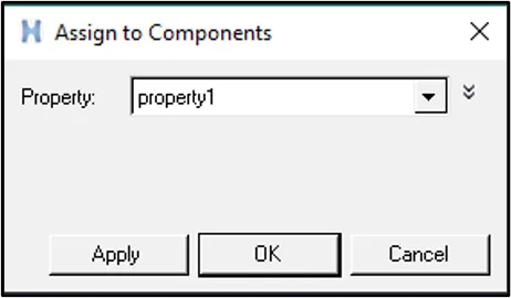
- Now assign the property to the required components.
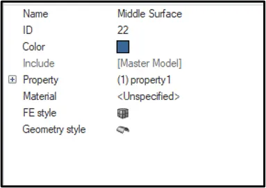
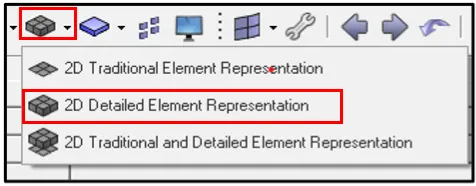
- Now, change the representation to 2D Detailed element representation.

Result:
For the above model, Midsurface was extracted and Meshing was done taking into account all the quality criterias and also assigning thickness to the elements.
Conclusion:
From the above Model we can conclude that before meshing, the model must be studied well that is all the geometrical errors must be cleared and then the midsurface must be extracted. During meshing, all the meshing rules muts be followed, clearing all the given qaulity criterias.
Final model: