Project 2
Aim: To develop a P1 hybrid model in simulink:
Hybrid vehicles:
Hybrid electric vehicles are powered by an internal combustion engine and one or more electric motors, which uses energy stored in batteries. A hybrid electric vehicle cannot be plugged in to charge the battery. Instead, the battery is charged through regenerative braking and by the internal combustion engine.
Four types of Hybrid Vehicles:
Mild Hybrids
One of the newest innovations in hybrid technology is that of a “mild” hybrid system. Like the name implies, a mild hybrid system typically isn’t going to propel the vehicle on electric power alone. Instead, the system is used to give a small boost to the vehicle’s gasoline engine, typically upon acceleration from a dead stop, and to assist in removing the burden of power-hungry systems, such as air conditioning, on the gasoline engine. Normally found in the form of 48 volt electric systems, mild hybrids do not need to be plugged in. Instead, the batteries are recharged through a combination of power from the gasoline engine, and energy recovered when the vehicle brakes (also known as regenerative brakes).
Mild hybrid systems go by many differing names, but some common examples are eAssist (General Motors), eTorque (Fiat/Chrysler), and EQ Boost (Mercedes).
Full Hybrids
Like mild hybrids, full hybrid vehicles also come equipped with both a gasoline engine and an electrical component. However, the electrical component in a full hybrid vehicle is capable of handling far more of the workload than that of a mild hybrid. Most full hybrids can actually operate for some distance solely on electric power. This typically happens at lower city speeds, but is one reason why you may see a full hybrid’s City MPG rating higher than its Highway MPG rating (where in standard gasoline-powered vehicles, the opposite is true).
When it comes to full hybrid vehicles, there are two main types of powertrains; Parallel hybrids and Series hybrids.
In Parallel hybrids, the engine can be powered in one of 3 ways: directly by the engine, directly by the electrical motor, or by both systems working together.
In a Series hybrid, the wheels are powered solely via the electric motor, with the gasoline-engine providing power for the electric motor, sort of like a generator. The gasoline-engine never actually powers the wheels.
With advances in hybrid technology, some vehicles operate as a combination of the two (aptly named “series-parallel” hybrids), with the on-board computer system choosing the most efficient way to operate at any given time.
Full hybrids charge their battery system in essentially the same way as mild hybrid systems, through energy from the gasoline engine as well as regenerative braking.
Plug-In Hybrids
All of the hybrid vehicles that we have discussed thus far charge their batteries solely through internal means. The main difference with plug-in hybrids is that these vehicles can charge their batteries via external chargers as well as internal. As a result, plug-in hybrids usually have greater electric-only ranges than full hybrids. Plug-In hybrids essentially serve as a half-way point between full hybrid vehicles and fully electric vehicles.
Electric Vehicles with Range Extender Hybrids
While all-electric vehicles technically don’t qualify as hybrids, there are some that come equipped with a small gasoline engine to provide a cushion when needed. When an electric vehicle runs out of power, the vehicle will need to be charged before it becomes operational again. These range extender hybrids utilize their gasoline engine to charge the battery or power the electric motor so that you’re not left stranded. Depending on the size of the gasoline engine, this can mean anywhere from a few dozen kms to hundreds.
Another classification of hyvrid vehicles:
PO hybrid belt driven moto generator.
P1 hybrid after engine flywheel.
P2 hybrid downstream of a disconnection clutch.
P3 hybrid after the gear.
P4 hybrid on the rear axle.
P5 hybrid in the wheels.
To run the simulation of the vehicle using matlab and simulink we define the variables in the amtlab workspace using the initialisation file where in we define the variables used in the simulink model.
The following is the matlab initialisation file:
%%%%%%%%%%%%%%%%%%%%%%%%%%%%%%%%%%%%%%%%%%%%%%%%%%%%%%%%%%%%%%%%%%%%%
%% Skill-Lync -> Hybrid Drives Development
% Project 1 - Conventional Vehicle Model
% By - Ullekh Gambhira

% Description:

%% Initialization File
% Initialization file for loading the variables for the Conventional vehicle simulation model

%% Vehicle Parameters
M = 1500;       % Vehicle weight [kg]
Cr = 0.015;     % Rolling resistance coefficient
Rw = 0.35;      % Rolling radius [m]
Cd = 0.33;      % Drag coefficient
Af = 2;         % Frontal area [m2]
rhoa = 1.225;   % Air density [kg/m3]
Vwind = 0;      % Wind velocity [kmph]
g = 9.81;       % Gravitational acceleration [m/s2]
theta = 0;      % Slope [deg]
myu_road_tire = 1; % Coefficient of friction between tire - road interface

%% Powertrain Parameters
FDR = 3.73;                         % Final Drive Ratio / Diff Ratio
DiffEff = 0.99;                     % Differential efficiency (assumed independent of operating conditions)

NumGear = 4;                        % Number of gears in transmission
TransGear = [1:NumGear];            % Transmission Gears
TransRatio = [3.06, 1.62, 1, 0.7];  % Corresponding Transmission ratios
TransEff = 0.90;                    % Transmission efficiency (assumed independent of operating conditions)

TC_SR = [0, .5, .6, .7, .8, .87, .92, .94, .96, .97, 1];   % Torque Converter Speed Ratio (Matlab default) -> TurbSpd/PumpSpd
TC_TR = [2.232, 1.5462, 1.4058, 1.2746, 1.1528, 1.0732, 1.0192, 1, 1, 1, 1];   % Torque Converter Torque Ratio (Matlab default) -> TurbTrq/PumpTrq
TC_Cf = 1e-4 * [.72558, .66322, .63463, .59042, .51331, .4144, .29287, .22444, .12186, .04386, 0]; % Torque Converter Capacity Factor (Matlab default) -> PumpTrq/PumpSpd^2 [Nm/rpm^2]

load Vehicle_Data/Engine_data_1_9L_Saturn_95kW
load Vehicle_Data/Trans_Shift_map
load Vehicle_Data/EM_Honda_Insight_10kW
load Vehicle_Data/ESS_NiMH6


ESS_init_soc = 0.8;
ESS_soc_max = 0.9;
ESS_soc_min = 0.6;


%% Driver Parameters
Kp = 10;                    % P gain for driver PI model
Ki = 1;                     % I gain for driver PI model
Drive_Cycle_Select = 1;     % Drive cycle selection

% Drive cycle values in m/s

if Drive_Cycle_Select == 1
    load DriveCycles/UDDS;

elseif Drive_Cycle_Select == 2
    load DriveCycles/HWFET;

elseif Drive_Cycle_Select == 3
    load DriveCycles/FTP;

elseif Drive_Cycle_Select == 4
    load DriveCycles/US06;

elseif Drive_Cycle_Select == 5
    load DriveCycles/NEDC;

elseif Drive_Cycle_Select == 6
    load DriveCycles/WLTP;

end

time_end = cyc_time(end);
vel_end = cyc_vel(end);
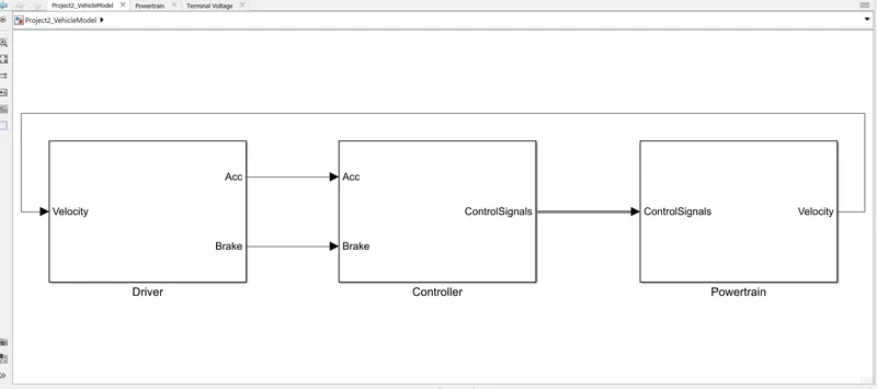
The simulink model of the p1 hybrid vehicle is follows:
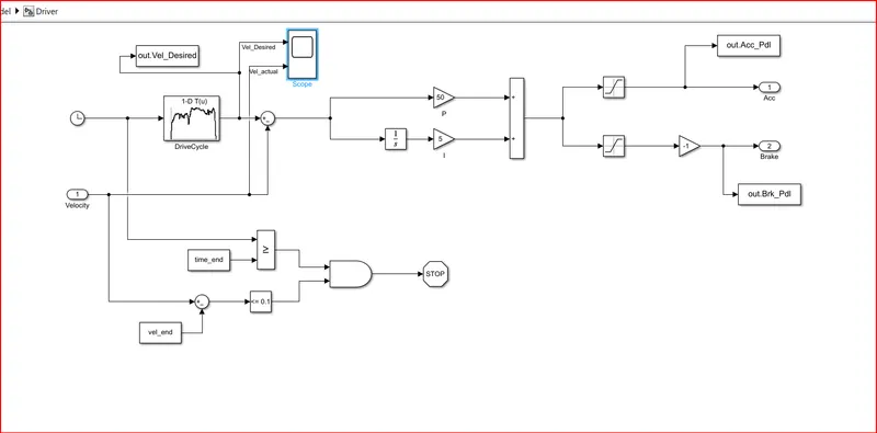
Driver block:
Controller block:
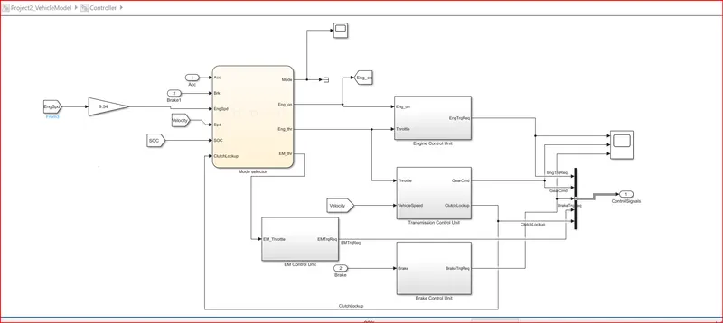
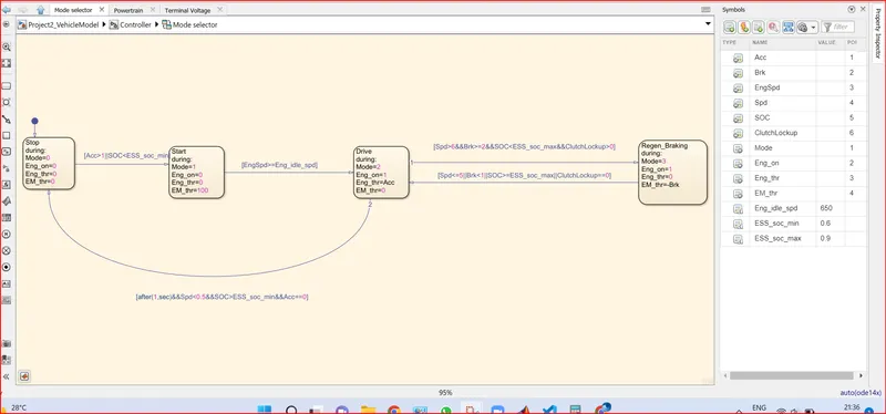
Mode controller block:
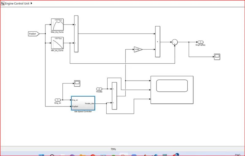
Engine control unit:
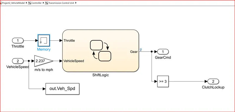
Transmission control unit:
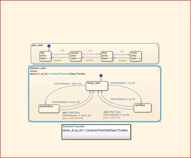
Shift logic used in transmission control unit:
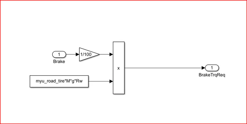
Brake control unit:
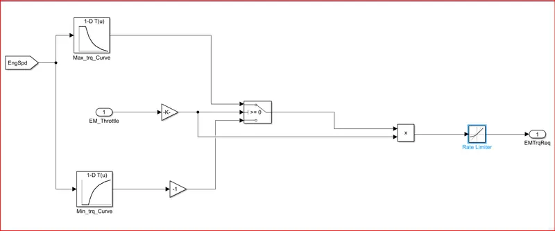
EM control uint:
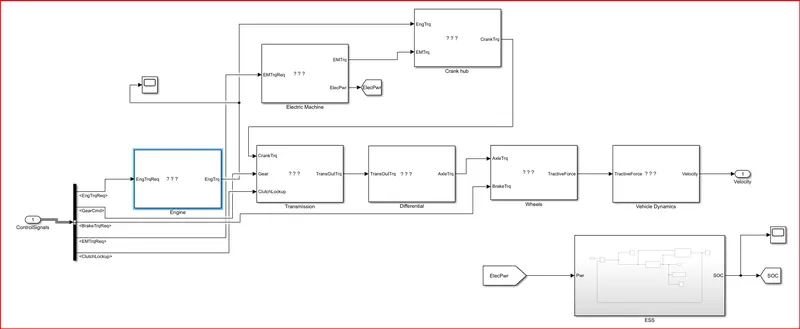
Powertrain block:
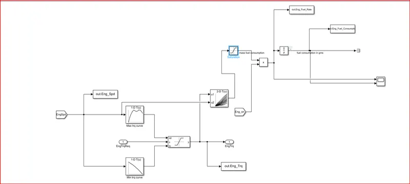
Engine block:
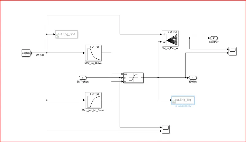
Electrical motor block:
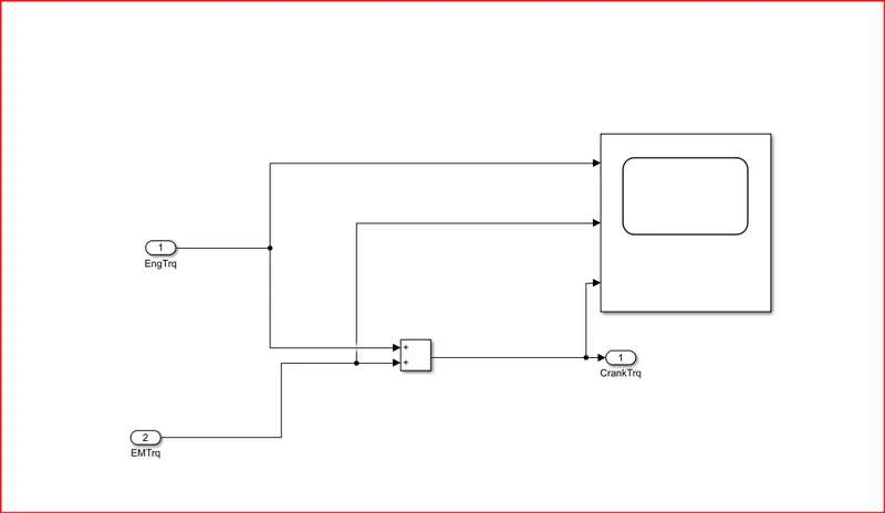
Crank hub:
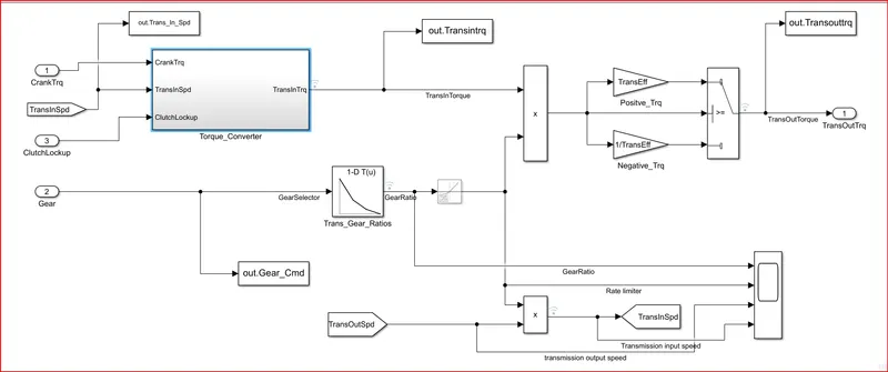
Transmission block:
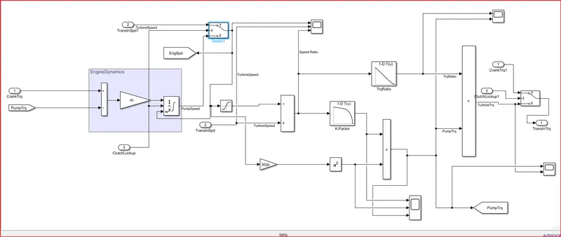
Torque converter:
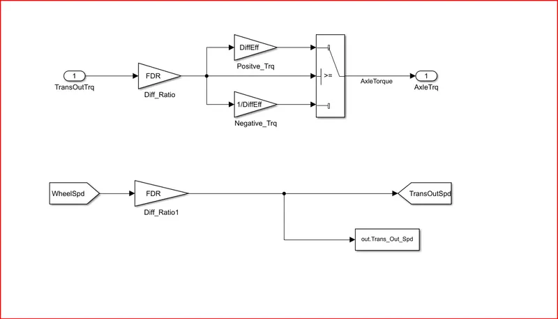
Differential:
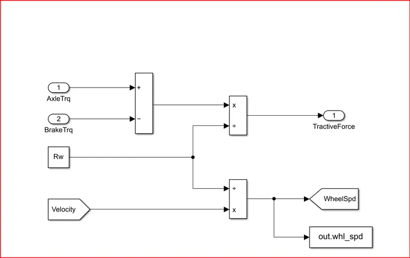
Wheels:
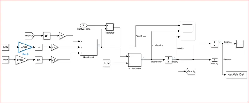
Vehicle dynamics:
ESS:
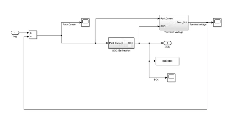
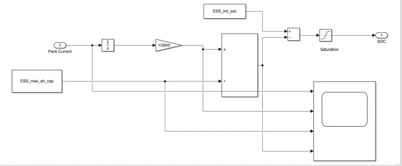
SOC Estimation:
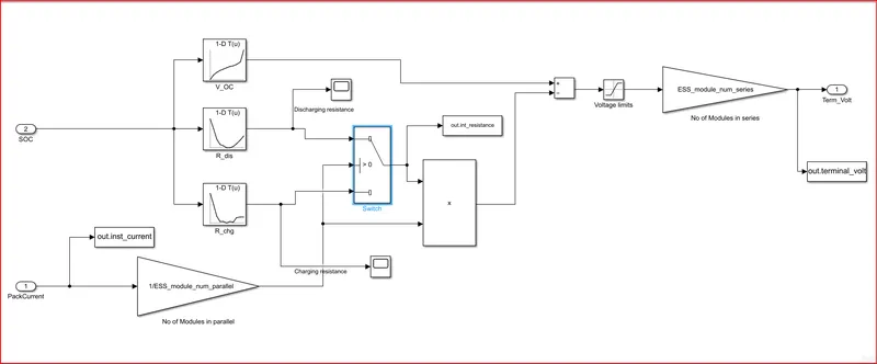
Terminal voltage:
Matlab processing file to generate the given plots:
Time = out.tout;
Acc_Pdl = out.Acc_Pdl;          % Accelerator pedal [%]
Brk_Pdl = out.Brk_Pdl;          % Brake pedal [%]
Gear_Cmd = out.Gear_Cmd;        % Transmission gear
Trans_In_Spd = out.Trans_In_Spd*30/pi;  % Transmission input speed [rpm]
Trans_Out_Spd = out.Trans_Out_Spd*30/pi;% Transmission output speed [rpm]
Eng_Trq = out.Eng_Trq;          % Engine brake torque [Nm]
Eng_Spd = out.Eng_Spd*30/pi;    % Engine speed [rpm]
Eng_Fuel_Consump = out.Eng_Fuel_Consumption;    % Engine fuel consumption [g]
Eng_Fuel_Rate = out.Eng_Fuel_Rate;   %engine fuel rate
Veh_Dist = out.Veh_Dist/1000;   % Distance traveled by vehicle [km]
Veh_Spd = out.Veh_Spd*18/5;     % Vehicle speed [kmph]
Whl_Spd = out.whl_spd*30/pi;     % wheel speed[RPM]
Desired_spd = out.Vel_Desired*18/5 ;  %desired speed [KMPH]
EM_Spd = out.EM_Spd*30/pi;         % E motor speed[rpm]
EM_Trq = out.EM_Trq;               % E motor torque[Nm]
EM_Pwr = out.EM_Pwr;               % E motor input power[W]
V_batt = out.V_battery;              % battery pack voltage [V]
I_batt = out.I_battery;              % battery pack current [I]
SOC = out.SOC;                     % STATE OF CHARGE [%]
RS = out.RS;                       % internal resistance
VOC = out.VOC;                     % open circuit voltage

%% Data Analysis
Eng_Pwr = Eng_Spd.*pi/30.*Eng_Trq/1000;   % Engine brake power [kW]
rho_petrol = 0.7197;                    % Density of petrol [kg/L]
kmpl = Veh_Dist(end)/(Eng_Fuel_Consump(end)/1000/rho_petrol);    % Fuel economy [kmpl];


% display fuel Economy of the cycle
formatspec = 'fuel economy is %2.2f kmpl';
fprintf(formatspec,kmpl);


%% Plotting vehicle characteristics time trace

% ploting transmission input,transmission output and wheel speed
figure(1)
hold on
grid on
plot(Time,Trans_In_Spd,'LineWidth',1,'Color','black');
plot(Time,Trans_Out_Spd,'LineWidth',1,'Color','red');
plot(Time,Whl_Spd,'LineWidth',1,'Color','blue');
xlabel('Time[s]')
ylabel('speed[rpm]')
xlim([0,Time(end)]);
legend('trans input','trans Output','wheel speed');
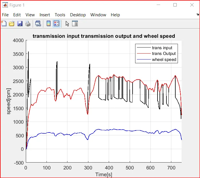
title('transmission input transmission output and wheel speed')

% plotting engine torque,engine power,fuel rate ,fuel consumption
figure(2)
subplot(4,1,1)
hold on
grid on
plot(Time,Eng_Trq,'LineWidth',1,'Color','black');
ylabel('torque[NM]')
xlim([0,Time(end)]);
title('Engine Torque')

subplot(4,1,2)
hold on
grid on
plot(Time,Eng_Pwr,'LineWidth',1,'Color','black');
ylabel('power[KW]')
xlim([0,Time(end)]);
title('Engine Power')

subplot(4,1,3)
hold on
grid on
plot(Time,Eng_Fuel_Rate,'LineWidth',1,'Color','black');
xlim([0,Time(end)]);
xlabel('Time[s]');
ylabel('Engine fuel rate');
title('Engine fuel rate')

subplot(4,1,4)
hold on
grid on
plot(Time,Eng_Fuel_Consump,'LineWidth',1,'Color','black');
xlim([0,Time(end)]);
xlabel('Time[s]');
ylabel('Engine fuel consumption[g]');
title('Engine Fuel Consumption')

% plotting accelerator and brake pedal gear command vehicle desired and actual speed ,vehicle distance
figure(3)

subplot(4,1,1)
hold on
grid on
plot(Time, Acc_Pdl, 'linewidth', 1, 'Color', 'black');
plot(Time, Brk_Pdl, 'linewidth', 1, 'Color', 'red');
ylabel('Pedal [%]')
xlim([0, Time(end)]);
legend('Accel','Brake');
title('Acceleration and brake pedal inputs')

subplot(4,1,2)
hold on
grid on
plot(Time, Gear_Cmd, 'linewidth', 1, 'Color', 'black');
xlim([0, Time(end)]);
xlabel('Time [s]');
ylabel('Gear');
title('gear command')

subplot(4,1,3)
hold on
grid on
plot(Time, Veh_Spd, 'linewidth', 1, 'Color', 'black');
plot(Time, Desired_spd, 'linewidth', 1, 'Color', 'red');
ylabel('Speed [kmph]')
xlim([0, Time(end)]);
legend('actual speed','desired speed');
title('vehicle actual and desired speed')

subplot(4,1,4)
hold on
grid on
plot(Time, Veh_Dist, 'linewidth', 1, 'Color', 'black');
xlim([0, Time(end)]);
xlabel('Time [s]');
ylabel('distance[km]');
title('vehicle distance')

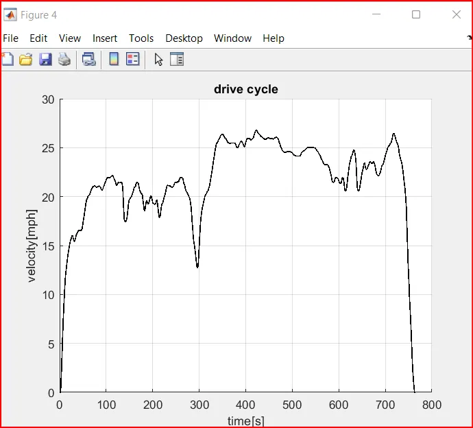
% plotting drive cycle
figure(4)
hold on
grid on
plot(cyc_time,cyc_vel,'LineWidth',1,'Color','black')
xlabel('time[s]')
ylabel('velocity[mph]')
title('drive cycle')


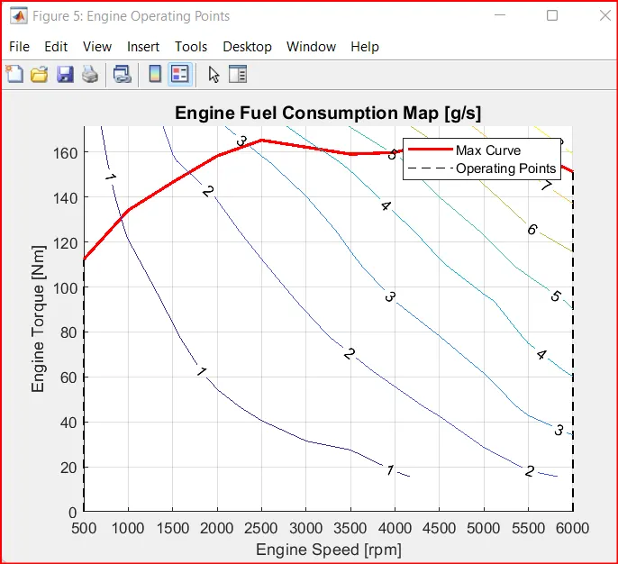
%% Plotting engine operating points on engine fuel map
figure('Name','Engine Operating Points');
hold on
grid on
title('Engine Operating Points','fontsize',12);
plot(Eng_map_spd*30/pi,Eng_max_trq,'linewidth',2,'color','r');
p2=line([Eng_map_spd(end)*30/pi Eng_map_spd(end)*30/pi],[0 Eng_max_trq(end)]);
set(p2,'linewidth',1,'linestyle','--','color','k');
p3=line([Eng_map_spd(1)*30/pi Eng_map_spd(1)*30/pi],[0 Eng_max_trq(1)]);
set(p3,'linewidth',1,'linestyle','--','color','k');
[c,h] = contour(Eng_map_spd'*30/pi,Eng_map_trq,Eng_fuel_map');
clabel(c,h);
xlabel('Engine Speed [rpm]');
ylabel('Engine Torque [Nm]');
title('Engine Fuel Consumption Map [g/s]');
legend({'Max Curve','Operating Points'});
axis([Eng_map_spd(1)*30/pi Eng_map_spd(end)*30/pi 0 Eng_map_trq(end)]);

%% Electric Motor
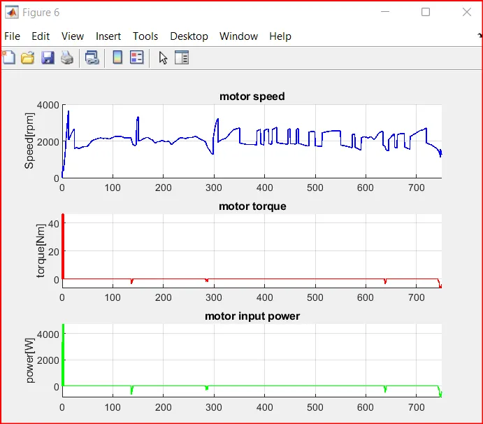
% plotting motor speed ,motor torque,motor input power

figure(6)
subplot(3,1,1)
hold on
grid on
plot(Time,EM_Spd,'LineWidth',1,'Color','b');
ylabel('Speed[rpm]')
xlim([0,Time(end)]);
title('motor speed')

subplot(3,1,2)
hold on
grid on
plot(Time,EM_Trq,'LineWidth',1,'Color','r');
ylabel('torque[Nm]')
xlim([0,Time(end)]);
title('motor torque')

subplot(3,1,3)
hold on
grid on
plot(Time,EM_Pwr,'LineWidth',1,'Color','g');
ylabel('power[W]')
xlim([0,Time(end)]);
title('motor input power')

%% BATTERY
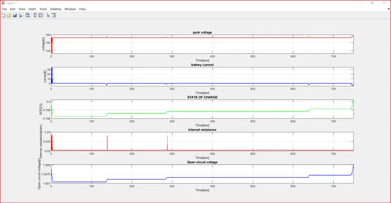
% plotting pack current,voltage,soc,internal resistance,open circuit
% voltage

figure(7)

subplot(5,1,1)
plot(Time,V_batt,'LineWidth',1,'Color','r');
xlabel('Time[sec]');
ylabel('voltage[v]');
title('pack voltage')
xlim([0,Time(end)]);
grid on

subplot(5,1,2)
plot(Time,I_batt,'LineWidth',1,'Color','b');
xlabel('Time[sec]');
ylabel('current[I]');
title('battery current')
xlim([0,Time(end)]);
grid on

subplot(5,1,3)
plot(Time,SOC,'LineWidth',1,'Color','g');
xlabel('Time[sec]');
ylabel('SOC[%]');
title('STATE OF CHARGE')
xlim([0,Time(end)]);
grid on

subplot(5,1,4)
plot(Time,RS,'LineWidth',1,'Color','r');
xlabel('Time[sec]');
ylabel('Internal resistance[ohm]');
title('Internal resistance')
xlim([0,Time(end)]);
grid on

subplot(5,1,5)
plot(Time,VOC,'LineWidth',1,'Color','b');
xlabel('Time[sec]');
ylabel('Open circuit voltage[v]');
title('Open circuit voltage')
xlim([0,Time(end)]);
grid on

%% Plotting engine operating points on engine fuel map
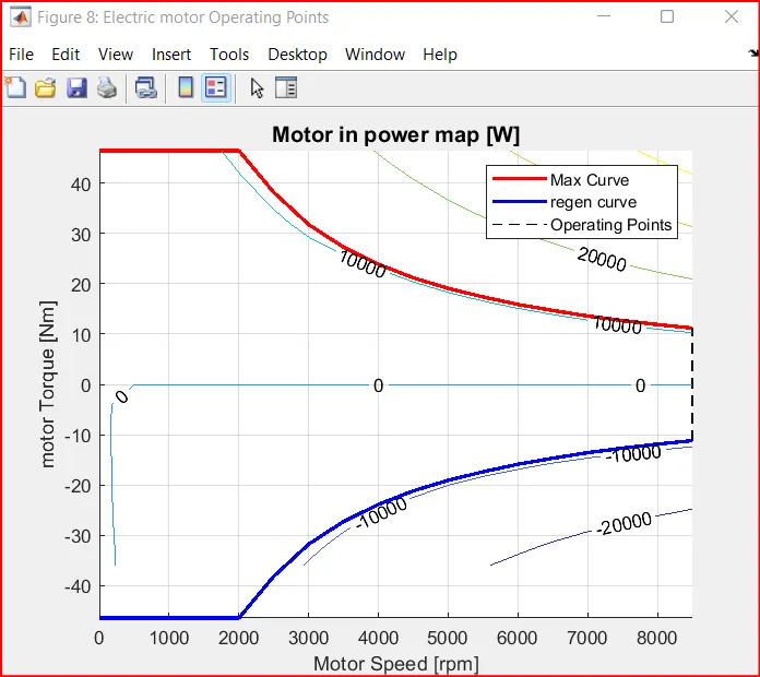
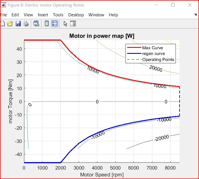
figure('Name','Electric motor Operating Points');
hold on
grid on
title('Electric motor Operating Points','fontsize',12);
p1=plot(EM_map_spd*30/pi,EM_max_trq,'linewidth',2,'color','r');
p4=plot(EM_map_spd*30/pi,EM_max_gen_trq,'LineWidth',2,'Color','b');
p2=line([EM_map_spd(end)*30/pi EM_map_spd(end)*30/pi],[EM_max_gen_trq(end) EM_max_trq(end)]);
set(p2,'linewidth',1,'linestyle','--','color','k');
p3=line([EM_map_spd(1)*30/pi EM_map_spd(1)*30/pi],[EM_max_gen_trq(1) EM_max_gen_trq(1)]);
set(p3,'linewidth',1,'linestyle','--','color','k');
[c,h] = contour(EM_map_spd'*30/pi,EM_map_trq,EM_inpwr_map');
clabel(c,h);
xlabel('Motor Speed [rpm]');
ylabel('motor Torque [Nm]');
title('Motor in power map [W]');
legend([p1 p4 p3],{'Max Curve','regen curve','Operating Points'});
xlim([EM_map_spd(1)*30/pi EM_map_spd(end)*30/pi]);
ylim([EM_max_gen_trq(1) EM_max_trq(1)]);
for UDDS cycle.
a. Tabulate the fuel economy numbers (kmpl) for UDDS and HWFET cycle. Compare these numbers with the baseline numbers for conventional vehicle model from Project 1.
fuel economy numbers (kmpl) for UDDS cycle is =13.3752 kmpl.
b. Plot the time trace for engine, transmission input, transmission output and wheel speed on one plot.
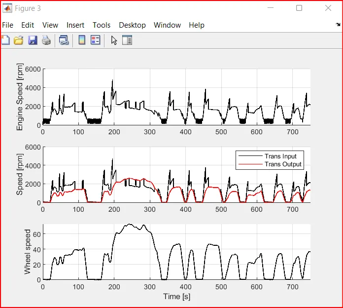
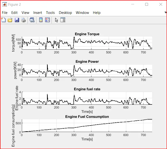
c. Plot engine torque, engine power, fuel rate and fuel consumption using subplots.
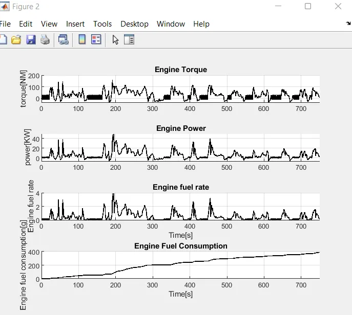
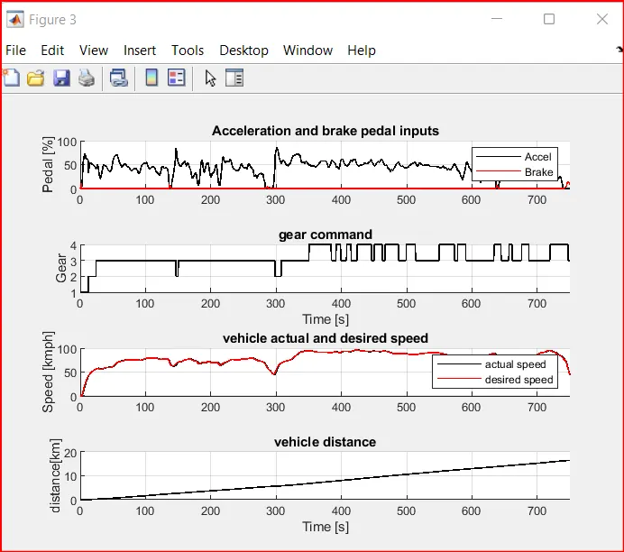
d. Plot accelerator and brake pedal, gear command, vehicle desired and actual speed, vehicle distance using subplots.
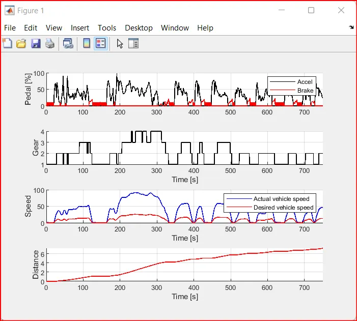
e. Plot the engine operating points on the engine fuel map.
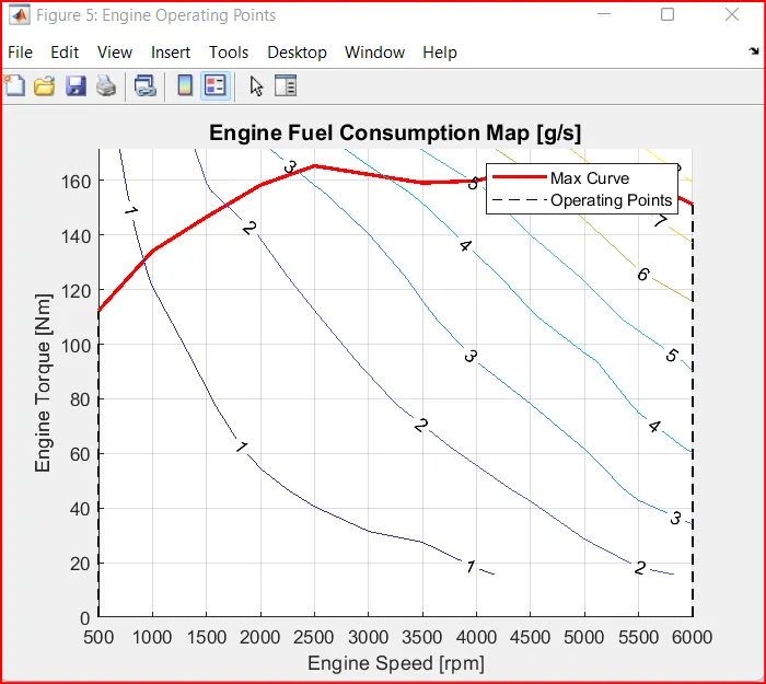
f. Plot motor speed, torque, motor input power using subplots.
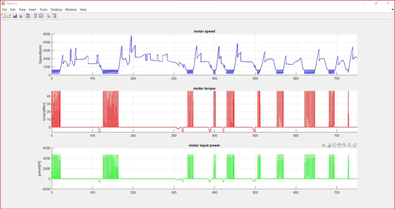
g. Plot pack voltage, current and SoC using subplots.
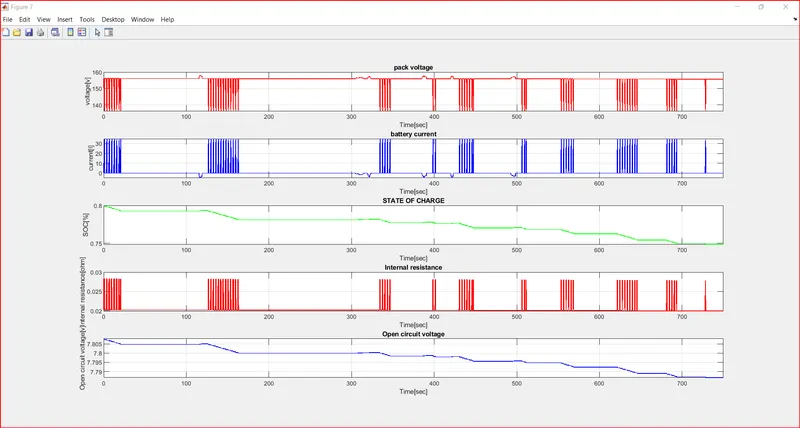
h. Plot the motor operating points on the motor input power map, with the motor max motoring and generating torque curves.
for HWFET cycle.
a. Tabulate the fuel economy numbers (kmpl) for UDDS and HWFET cycle. Compare these numbers with the baseline numbers for conventional vehicle model from Project 1.
fuel economy numbers (kmpl) for HWFET cycle is =16.91 kmpl.
b. Plot the time trace for engine, transmission input, transmission output and wheel speed on one plot.
c. Plot engine torque, engine power, fuel rate and fuel consumption using subplots.
d. Plot accelerator and brake pedal, gear command, vehicle desired and actual speed, vehicle distance using subplots.
e. Plot the engine operating points on the engine fuel map.
f. Plot motor speed, torque, motor input power using subplots.
g. Plot pack voltage, current and SoC using subplots.
h. Plot the motor operating points on the motor input power map, with the motor max motoring and generating torque curves.