Project 2
Project_02:Implement Clustering and then predict the class of car from “Car dataset”.
Attributes imformation:
1.symboling: -3, -2, -1, 0, 1, 2, 3
2.normalized-losses: continuous from 65 to 256
3.make: alfa-romero, audi, bmw, chevrolet, dodge, honda, isuzu, jaguar, mazda, mercedes-benz, mercury, mitsubishi, nissan, peugot, plymouth, porsche, renault, saab, subaru, toyota, volkswagen, volvo.
4.fuel-type: diesel, gas
5.aspiration: std, turbo
6.num-of-doors: four, two
7.body-style: hardtop, wagon, sedan, hatchback, convertible
8.drive-wheels: 4wd, fwd, rwd
9.engine-location: front, rear
10.wheel-base: continuous from 86.6 120.9
11.length: continuous from 141.1 to 208.1
12.width: continuous from 60.3 to 72.3
13.height: continuous from 47.8 to 59.8
14.curb-weight: continuous from 1488 to 4066
15.engine-type: dohc, dohcv, l, ohc, ohcf, ohcv, rotor
16.num-of-cylinders: eight, five, four, six, three, twelve, two
17.engine-size: continuous from 61 to 326
18.fuel-system: 1bbl, 2bbl, 4bbl, idi, mfi, mpfi, spdi, spfi
19.bore: continuous from 2.54 to 3.94
20.stroke: continuous from 2.07 to 4.17
21.compression-ratio: continuous from 7 to 23
22.horsepower: continuous from 48 to 288
23.peak-rpm: continuous from 4150 to 6600
24.city-mpg: continuous from 13 to 49
25.highway-mpg: continuous from 16 to 54
26.price: continuous from 5118 to 45400.
Importing neccessary libraries
import pandas as pd
import numpy as np
import matplotlib.pyplot as plt
import seaborn as sns
import warnings
warnings.filterwarnings('ignore')
Reading data
df1 = pd.read_csv('auto.csv')
df1.head()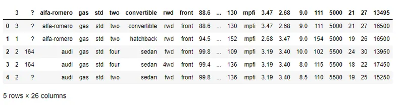
- In above dataframe the column names are not meaningfull and dadaset contains special characters.
Data Cleaning
Reading the data with proper column name and replacing special characters with NaN values
df = pd.read_csv('auto.csv',header = None,names = ['symboling','normalized-losses','make','fuel-type','aspiration','num-of-doors','body-style','drive-wheels','engine-location','wheel-base','length','width','height','curb-weight','engine-type','num-of-cylinders','engine-size','fuel-system','bore','stroke','compression-ratio','horsepower','peak-rpm','city-mpg','highway-mpg','price'],na_values=['?','??'])

df.head()
print(list(df.columns)) #Ckecking column names['symboling', 'normalized-losses', 'make', 'fuel-type', 'aspiration', 'num-of-doors', 'body-style', 'drive-wheels', 'engine-location', 'wheel-base', 'length', 'width', 'height', 'curb-weight', 'engine-type', 'num-of-cylinders', 'engine-size', 'fuel-system', 'bore', 'stroke', 'compression-ratio', 'horsepower', 'peak-rpm', 'city-mpg', 'highway-mpg', 'price']
df.info() #checking info 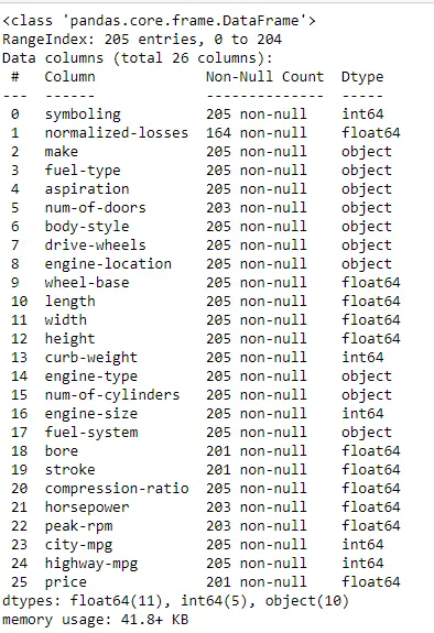
Handling missing values
#check missing values
df.isnull().sum()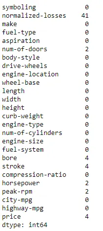
Replacing Missing Values with respective column mean
df['normalized-losses'].fillna(df['normalized-losses'].mean(),inplace=True)
df['bore'].fillna(df['bore'].mean(),inplace=True)
df['stroke'].fillna(df['stroke'].mean(),inplace=True)
df['horsepower'].fillna(df['horsepower'].mean(),inplace=True)
df['peak-rpm'].fillna(df['peak-rpm'].mean(),inplace=True)
df['price'].fillna(df['price'].mean(),inplace=True)
Replacing all null values in num-of-doors with four(majority) because categorical column.
df['num-of-doors'].value_counts()
df['num-of-doors'].fillna('four',inplace=True)
four 114 two 89 Name: num-of-doors, dtype: int64
Correcting datatypes
1.If we check in above Dtypes of all attribues,Some of attributes such as num-of- doors,num-of cylinder.
they should be 'int'or 'float' format instead of 'object'
2.So let's first convert the str to number using replace() and then convert the object to int or float uaing astype().
#Checking unique values of num-of-doors

df['num-of-doors'].unique()
array(['two', 'four'], dtype=object)
#replacing str to number
df['num-of-doors'].replace('two',2,inplace=True)
df['num-of-doors'].replace('four',4,inplace=True)
#converting object dtype value into int64
df['num-of-doors']=df['num-of-doors'].astype('int64')df['num-of-cylinders'].unique()array(['four', 'six', 'five', 'three', 'twelve', 'two', 'eight'],
dtype=object)
df['num-of-cylinders'].replace('two',2,inplace=True)
df['num-of-cylinders'].replace('three',3,inplace=True)
df['num-of-cylinders'].replace('four',4,inplace=True)
df['num-of-cylinders'].replace('five',5,inplace=True)
df['num-of-cylinders'].replace('six',6,inplace=True)
df['num-of-cylinders'].replace('eight',8,inplace=True)
df['num-of-cylinders'].replace('twelve',12,inplace=True)

df['num-of-cylinders']=df['num-of-cylinders'].astype('int64')
Binning:
- Binning:Binning is a process of transforming continuous numerical variables into discrete categorical 'bins', for grouped analysis.
df['horsepower'].describe()
df["horsepower"] = df["horsepower"].astype(int, copy=True)

#Copy = True willl create the another copy of column including changes to it.
#int is Dtype we want apply.

df["horsepower"]
Histogram of horsepower
plt.hist(df['horsepower'])
#Setting x&y labels
plt.xlabel("horsepower")
plt.ylabel("count")
plt.title("horsepower bins")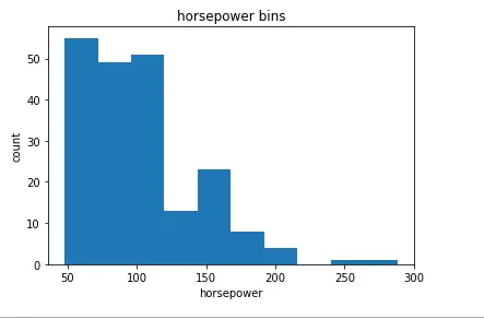
- 3 bins of equal size bandwidth so we use numpy's linspace(start_value, end_value, numbers_generated function.
- Since we are building 3 bins of equal length, there should be 4 dividers, so numbers_generated=4.
bins = np.linspace(min(df["horsepower"]),max(df["horsepower"]),4)
bins
array([ 48., 128., 208., 288.])
bins_names = ['Low', 'Medium', 'High']df['horsepower-binned'] = pd.cut(df['horsepower'], bins, labels=bins_names ,include_lowest = True)
#df[['horsepower','horsepower-binned']].head(5)
df['horsepower-binned']=df['horsepower-binned'].astype('object')
#df["horsepower-binned"].value_counts()
#let's drop the horsepower column
df.drop(['horsepower'],axis=1,inplace=True)
df.head()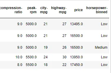
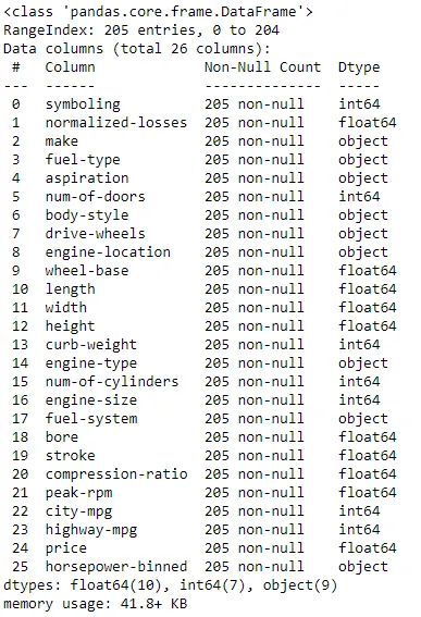
- Till now we have cleaned data, by removing NaN values and special characters and proper naminng to columns
Exploring data with visvulization
df.shape
df.info()
(205, 26)
df.describe().T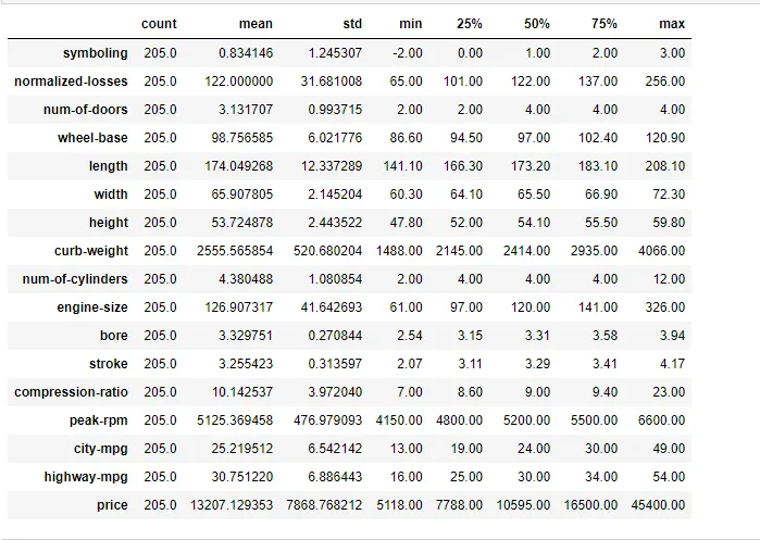
Countplots
cat_list = ['symboling','num-of-doors', 'num-of-cylinders','fuel-type', 'aspiration', 'body-style', 'drive-wheels', 'engine-location', 'horsepower-binned']
fig, axs = plt.subplots(nrows=4,ncols=2,figsize =(15,20))
for col,ax in zip(cat_list[0:],axs.ravel()):
    sns.countplot(x=col,data=df,ax=ax)
    plt.xticks(rotation='vertical')
    plt.savefig("Countplot",facecolor='y',bbox_inches="tight",pad_inches=0.3, transparent=True)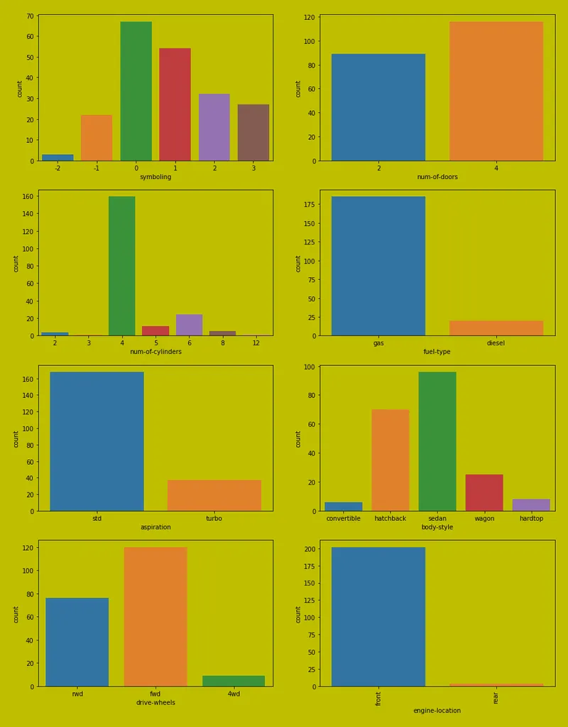
- 1.four doors are higher than the two doors cars.
- 2.maximum numbers of cars having four number of cylinders in them followed by 6 number of cylinders and then 5.
- 3.Most of the cars at working on gas.
- 4.most of the cars are front wheel drive.
- 5.Almost cars have engine located at front.
Barplot
df_make_count = df['make'].value_counts()

fig, ax = plt.subplots(1, 2, figsize=(20,10))
df_make_count_barplot = sns.barplot(y = df_make_count.index,x = df_make_count.values, ax = ax[0])
df_make_count_barplot.set_ylabel('count')
df_make_count_barplot.set_xlabel('Car brand')
df_make_count.plot.pie(autopct="%1.1f%%", ax=ax[1])
plt.savefig("vehicles count",facecolor='g', bbox_inches="tight",
            pad_inches=0.3, transparent=True)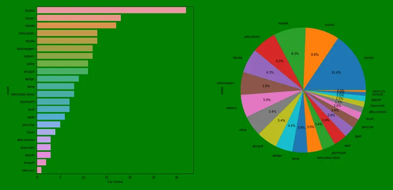
- we can see that most of the cars in the datasets is of toyota brand followed by nissan, mazda etc
df_make_count = df['fuel-system'].value_counts()

fig, ax = plt.subplots(1, 2, figsize=(20,10))
df_make_count_barplot = sns.barplot(x = df_make_count.index,y = df_make_count.values, ax = ax[0])
df_make_count_barplot.set_ylabel('count')
df_make_count_barplot.set_xlabel('fuel-system')
df_make_count.plot.pie(autopct="%1.1f%%", ax=ax[1])
plt.savefig("fuel-system",facecolor='g', bbox_inches="tight",
            pad_inches=0.3, transparent=True)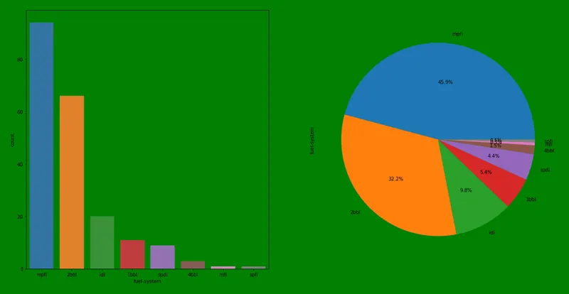
- Most of the Vehicles uses 'mpfi' fuel-injection system
df_make_count = df['engine-type'].value_counts()

fig, ax = plt.subplots(1, 2, figsize=(20,10))
df_make_count_barplot = sns.barplot(x = df_make_count.index,y = df_make_count.values, ax = ax[0])
df_make_count_barplot.set_ylabel('count')
df_make_count_barplot.set_xlabel('engine-type')
df_make_count.plot.pie(autopct="%1.1f%%", ax=ax[1])
plt.savefig("engine-type",facecolor='g', bbox_inches="tight",
            pad_inches=0.3, transparent=True)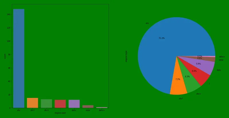
- Most of the vehicles have 'Ohc' type engine
Boxplot to detect outliers
num = [ 'normalized-losses', 'wheel-base', 'length', 'width', 'height', 'curb-weight', 'engine-size', 'bore', 'stroke', 'peak-rpm', 'price', 'city-mpg', 'highway-mpg']
fig, axs = plt.subplots(nrows=5,ncols=3,figsize =(15,20))
for col,ax in zip(num[0:],axs.ravel()):
    sns.boxplot(x=col,data=df,ax=ax)
    plt.xticks(rotation='vertical')
    plt.savefig("boxplot", bbox_inches="tight",
            pad_inches=0.3, transparent=True)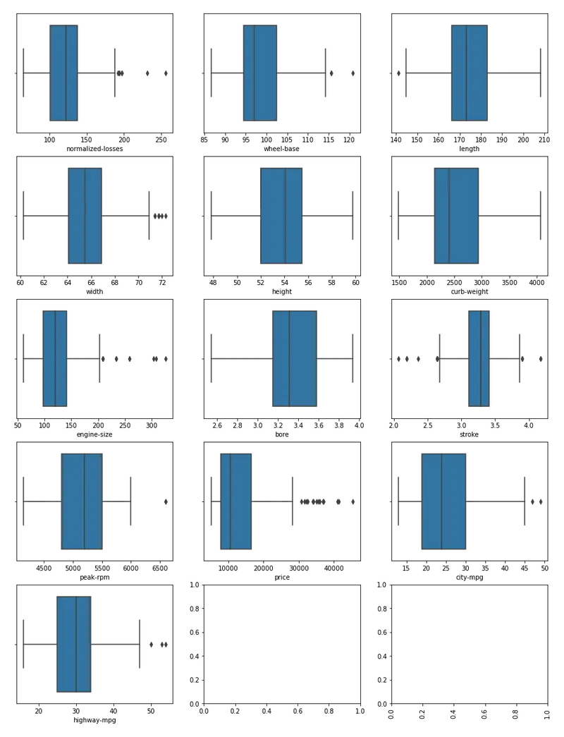
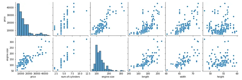
Pairplot between price and all other attributes
sns.pairplot(df,x_vars=["price","num-of-cylinders","engine-size","length","width","height"],y_vars=["price","engine-size"],)
Boxplots
- Categorical attributes and their correlation with price
sns.boxplot(x="body-style", y="price", data=df)
plt.savefig('body style vs price')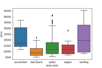
- Above we can see,boxes overlap and their median lines are inside the overlap range.
- As we mentioned above distributions of price between the different body-style categories have a significant overlap,and so body-style would not be a good predictor of price.
sns.boxplot(x="engine-location", y="price", data=df)
plt.savefig('location vs price')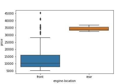
- two boxes are not overlaped and they are enough distinct, we can say engine location is the predictor of price
sns.boxplot(x="aspiration", y="price", data=df)
plt.savefig('aspiration vs price')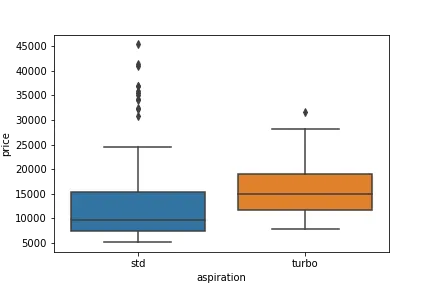
sns.boxplot(x="drive-wheels", y="price", data=df)
plt.savefig('Dw vs price')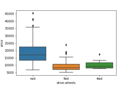
Correlation and Heatmap
df.corr()

plt.figure(figsize=(20,10))
sns.heatmap(df.corr(),annot=True)
plt.savefig('Heatmap')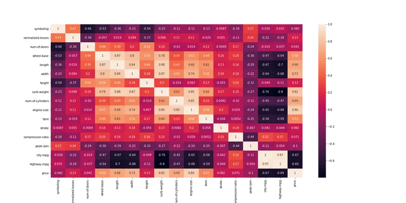
- Compression-ratio has very strong negative correlation with fuel-type
- Price has very strong positive relationship with curb-weight and engine size
- Engine size has positive relationship with num-of cylider,leght,width,height
Converting Categorical columns into Numerical column using labelEncoder
#Creating catagorical list
objList = df.select_dtypes(include = "object").columns
print (objList)
Index(['make', 'fuel-type', 'aspiration', 'body-style', 'drive-wheels',
'engine-location', 'engine-type', 'fuel-system', 'horsepower-binned'],
dtype='object')
from sklearn.preprocessing import LabelEncoder
le = LabelEncoder()

for i in objList:
    df[i] = le.fit_transform(df[i].astype(str))

#print (df.info())

df.head()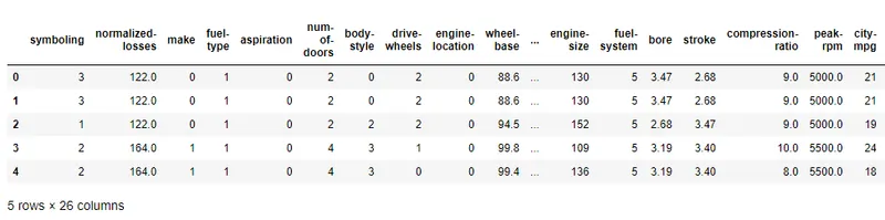
Standardizing data
from sklearn.preprocessing import StandardScaler
scaler = StandardScaler()
df1= pd.DataFrame(scaler.fit_transform(df),columns=df.columns)

df1.head()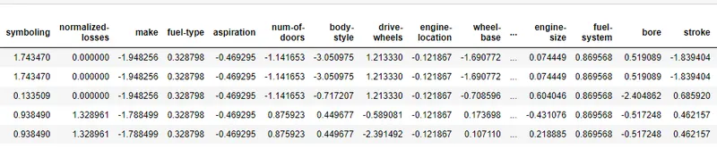
After standardization next step is to reduce some dimension using PCA technique
Implementing The Principal component analysis
from sklearn.decomposition import PCA
pca = PCA(n_components=3)
principalComponents = pca.fit_transform(df1)
Df = pd.DataFrame(data = principalComponents,columns = ['pc1','pc2','pc3'])
print(Df)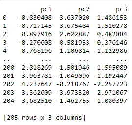
#Explained variance ratio

print(pca.explained_variance_ratio_)
[0.32361609 0.16496542 0.08762615] # It shows the percentage of variance that is attributed by each of the selected components i.e Pc1 has 32 %,pc2 %16.
Finding optimun value of K usinng elbow curve
from sklearn.cluster import KMeans

k_range = range(2,20)

sse = []
for k in k_range:
    km1=KMeans(n_clusters=k)
    km1.fit_predict(Df)
    sse.append(km1.inertia_)
plt.plot(k_range,sse,marker ='*')
plt.ylabel('SSE')
plt.xlabel('K_values')
plt.show() 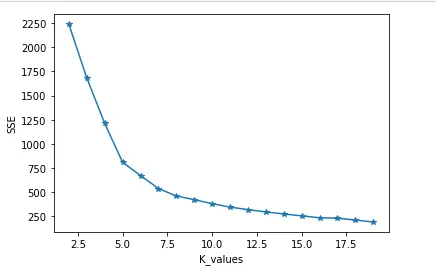
Applying KMean algorithm
km = KMeans(n_clusters=5)
print(km)
y= km.fit_predict(Df)
print(y)
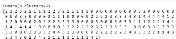
Df['Class']=y
df0 = Df[Df.Class==0]
df1 = Df[Df.Class==1]
df2 = Df[Df.Class==2]
df3 = Df[Df.Class==3]
df4 = Df[Df.Class==4]

Df.head()
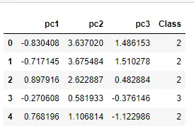
By using KMean we have created class,we can see in graph .
#Centroids

print(km.cluster_centers_)
[[-3.11498837 0.46531071 0.21172379] [ 3.90748089 -0.2902233 -1.22341231] [ 1.03594318 2.73158485 0.81878428] [-0.90740928 -1.02286722 -1.1820883 ] [ 1.70350465 -3.82299174 3.30010375]]
Cluster Visualization
plt.figure(figsize=(10,7))
a=plt.scatter(df0['pc1'],df0['pc2'],c='red')
b=plt.scatter(df1['pc1'],df1['pc2'],c='green')
c=plt.scatter(df2['pc1'],df2['pc2'],c='blue')
d=plt.scatter(df3['pc1'],df3['pc2'],c='black')
e=plt.scatter(df4['pc1'],df4['pc2'],c='cyan')
plt.scatter(km.cluster_centers_[:,0],km.cluster_centers_[:,1],s=200,c='purple',marker='*')
plt.title('pc1 vs pc2')
plt.xlabel('pc1(variance_explained:0.32)')
plt.ylabel('pc2(variance_explained:0.16)')
plt.show()
plt.savefig('cluster')
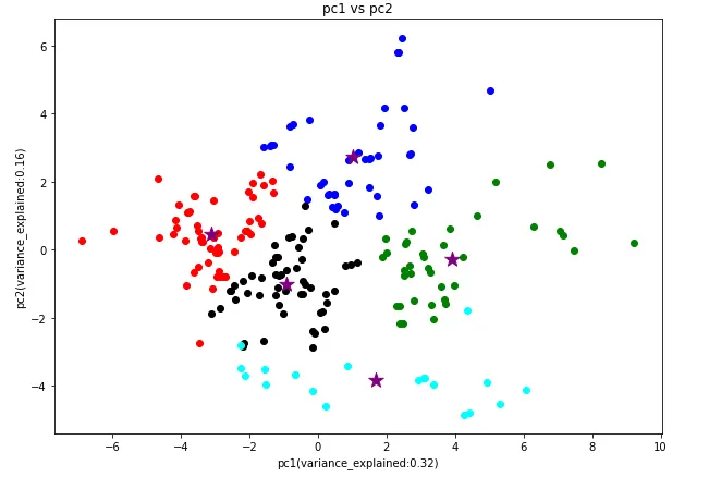
- Using Kmean wee have grouped data into 5 classes(clusturs).
- Next step is to predict class(clutures) using classification algorithms.
Predicting class using calssification model
Seperating independent and dependent features
x = Df.drop('Class',axis=1)
y = Df['Class']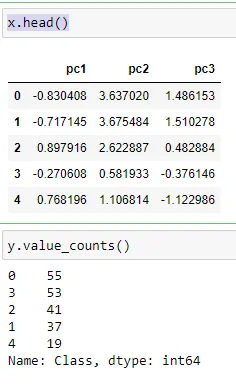
Splitting data into train and test
from sklearn.model_selection import cross_val_score
from sklearn.model_selection import train_test_split
X_train,X_test,Y_train,Y_test = train_test_split(x,y,test_size=0.3,random_state=0)
1.logistic regression
from  sklearn.linear_model import LogisticRegression
lr = LogisticRegression()
lr.fit(X_train,Y_train)
Y_p= lr.predict(X_test)
print("Logistic_Reg_train_score:",lr.score(X_train,Y_train))
print("Logistic_Reg_test_score:",lr.score(X_test,Y_test))
Logistic_Reg_train_score: 1.0 Logistic_Reg_test_score: 0.967741935483871
1.Ke-fold cross validation for logistic regression
score_lr=cross_val_score(lr,X_train,Y_train,cv=10)
print(score_lr)
print("Avg :",np.average(score_lr))
[1. 1. 0.93333333 0.92857143 1. 1. 1. 1. 1. 1. ] Avg : 0.9861904761904763
2.Support Vector Machine
from sklearn.svm import SVC
svm = SVC()
svm.fit(X_train,Y_train)
Y_pred_svm= svm.predict(X_test)
SVM_score = svm.score(X_test,Y_test)
print("SVM_train_score:",svm.score(X_train,Y_train))
print("SVM_test_score:",SVM_score)
SVM_train_score: 1.0 SVM_test_score: 0.9516129032258065
2.K-fold cross_validation for SVM
from sklearn.model_selection import cross_val_score
score_svm=cross_val_score(svm,X_train,Y_train,cv=10)
print(score_svm)
print("Avg :",np.average(score_svm))
SVM_train_score: 1.0 SVM_test_score: 0.9516129032258065
3.Decision Tree
from sklearn.tree import DecisionTreeClassifier
dtc = DecisionTreeClassifier()
dtc.fit(X_train,Y_train)
print("dtc_train_score:",dtc.score(X_train,Y_train))
print("dtc_test_score:",dtc.score(X_test,Y_test))
dtc_train_score: 1.0 dtc_test_score: 0.9032258064516129
3.K-fold cross_validation for decision tree
score_dtc=cross_val_score(dtc,X_train,Y_train,cv=10)
print(score_dtc)
print("Avg :",np.average(score_dtc))
[0.93333333 1. 1. 0.85714286 0.92857143 0.78571429 0.92857143 1. 1. 0.64285714]
Avg : 0.9076190476190475
4.Random forest
from sklearn.ensemble import RandomForestClassifier
rf = RandomForestClassifier(n_estimators=50,random_state=7)
rf.fit(X_train,Y_train)
Y_pred_rf= rf.predict(X_test)
print("rf_train_score:",rf.score(X_train,Y_train))
print("rf_test_score:",rf.score(X_test,Y_test))
rf_train_score: 1.0 rf_test_score: 0.967741935483871
Gap between train and test score is more.
4.K-fold cross validation random forest
score_rf=cross_val_score(rf,X_train,Y_train,cv=10)
print(score_rf)
print("Avg :",np.average(score_rf))
[1. 1. 0.86666667 0.92857143 0.92857143 0.85714286 1. 1. 1. 0.78571429]
Avg : 0.9366666666666668
5.KNN Classifier
from sklearn.neighbors import KNeighborsClassifier
knn = KNeighborsClassifier(n_neighbors=3)
knn.fit(X_train,Y_train)
print("Knn_train_score:",knn.score(X_train,Y_train))
print("Knn_test_score:",knn.score(X_test,Y_test))
Knn_train_score: 0.993006993006993 Knn_train_score: 0.9838709677419355
Gap between train and test accuarcy is very less as compare to other model
5.K-fold cross validation for Knn
from sklearn.model_selection import cross_val_score
score_knn=cross_val_score(knn,X_train,Y_train,cv=10)
print(score_knn)
print("Avg :",np.average(score_knn))
[1. 1. 0.86666667 1. 1. 1. 1. 1. 1. 1. ]
Avg : 0.9866666666666667
Accuracy comparision table
data = {'classifier':['Logistic_regression','SVM','Decision_tree','Random_forest','Knn'],
        'model_train_score':[1,1,1,1,0.99],
        'model_test_accuarcy ':[0.96,0.95,0.90,0.96,0.98],
        'k-fold_cross_score ':[0.98, 0.99,0.90,0.93,0.98]}


df2 = pd.DataFrame(data)
df2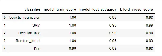
- from above table,
- For Knn classifier, the gap between train and test score is very less as compare to all other model.so Knn is performing very well.
- For logistic regression & random forest, gap between train and test is slightly more as compare to Knn.