Hybrid electric Vehicle model development using MATLAB and Simulink

Hybrid Vehicle model development using MATLAB and Simulink

1.AIM

To create a complete Hybrid Electric Vehicle model including Driver , Electric Power Train and Vehicle model.

Analyse the performance of the vehicle for a US06 drive cycle and plot the Actual velocity and Power distribution curves. Also analyse the performace and fuel consumption of fuel cell, Ultracapacitor and battery.

2.Objective

2.1 To observe the following plots of the Vehicle for the drive cycle.

1. Acceleration / Brake
2. Torque required
3. Power required
4. Power distribution among three energy sources
5. Fuel cell voltage, current, power and fuel consumption

2.2 Energy Management distribution algorithm for positive power distribution

The Energy management system implemented here will follow rule based algorithm for the implementation of series parallel hybrid systems.

The implementation algorithm and flow chart are explained below.

The operating range of the sources is as follows.

1. Battery
2. fuel

Figure : Flow chart for Positive Power Distribution

The flowchart for positive power distribution is as shown above.

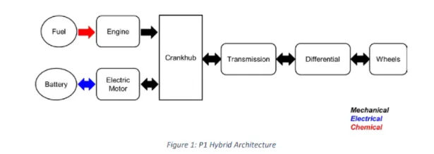
3. SIMULINK Modeling

The complete Simulink model of the vehicle is shown below. There are 3 main subsystems.

1. Driver 2. Electric power train 3. Vehicle

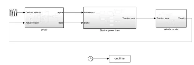
Figure : Basic vehicle model

Each of these subsystems modeling in Simulink is explained below.

3.1 Driver Model

The basic function of driver block is to generate Acceleration (Alpha) and Brake (Beta) signals according to Desired velocity and Actual velocity commands.

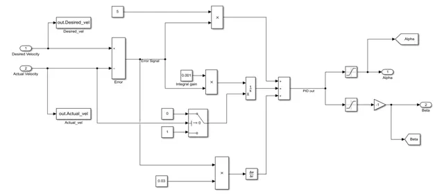
Figure : Driver

The input to the driver model is desired velocity and actual velocity. The desired velocity is the driving cycle input provided through a repeating sequence of which velocity and time profiles are declared in workspace. In our model, the input is given by US06 drive cycle. The US06 Supplemental Federal Test Procedure (SFTP) was developed to address the shortcomings with the FTP-75 test cycle in the representation of aggressive, high speed and/or high acceleration driving behavior, rapid speed fluctuations, and driving behavior following startup [15].

Actual velocity is the velocity of the vehicle which is taken as a feedback from output. The error signal which is the difference between desired and actual velocity is fed through a PID controller.

If the integral block does not reset properly, it may cause integral wind up problem. It occurs due to the limitation in actuators. The correction from the integral term of PID controller increases a lot which causes the system output to go beyond the set point. It is known as overshoot and it increases with time.

To avoid these problems, external reset is provided to the integral block. Whenever the velocity becomes zero, this integral block gets reset. It is implemented through a switch. It passes a zero to the integral block whenever velocity gets zero.

The output of the PID controller is fed to the saturation block to get positive values. The Alpha can have any value from 0 to 1 and Beta from 0 to -1. The values of PID controller are optimized by observing the output velocity and input velocity profiles.

3.1.1 Observation

When desired velocity > Actual velocity, Acceleration is ‘1’ and Brake is ‘0’.

If Desired velocity < Actual velocity, Acceleration is ‘0’ and Brake is ‘1’.

When both Desired and Actual velocities are same, Acceleration = Brake = 0

3.2 Electric Power Train

The Electric power train contains the following blocks.

1. Controller
2. Power Calculation
3. Tractive Force
4. EMS (Energy Management System)
5. UC model
6. Fuel cell
7. Battery model

The input/output signal arrangements inside ‘Electric power train’ subsystem is as shown below.

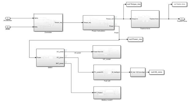
Figure : Electric Power Train

3.2.1 Controller

The controller block generates required torque signal from Acceleration and Brake commands. Electric motor torque (positive) values are declared in workspace as variable ‘EM_new.maxT_T’ array and negative values are declared as variable ‘EM_new.minT_T’ array.

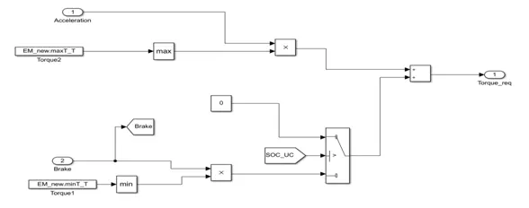
Figure : Controller

The Acceleration and brake outputs of ‘Driver’ subsystem is fed to ‘Controller’ block. The ‘max’ block will take the maximum value and ‘min’ block will take the minimum value.

The SOC of ultracapacitor is being checked for regenerative braking. If the SOC_UC > 0.8, then it won’t be further charged while braking. If the SOC_UC <0.8, then UC will get charged when braking occurs.

While Acceleration positive torque request will be generated and while braking, negative torque will be generated. This torque request is fed to ‘Power Calculation’ block.

3.2.2 Power Calculation

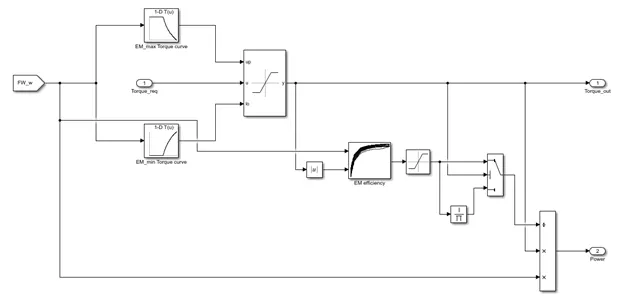
Figure : Power Calculation

This subsystem will calculate required power for a given angular velocity and Torque.

In order to calculate power, we need angular velocity, torque and efficiency.

Power = (Torque * Angular velocity) / Efficiency

3.2.2.1 Angular velocity (w)

Angular velocity of the wheel is calculated inside ‘Tractive force‘ block and fed to this block.

3.2.2.2 Torque

For a given acceleration/brake the required torque being calculated by ‘Controller’ subsystem and fed to the ‘Power calculation’ block. Inside this there is a dynamic saturation block which will check whether the required torque is in the limits of torque that can be supplied by the Electric Motor. This is done by comparing the ‘Torque req’ with two curves of ‘w’ Vs ‘Torque’. Where ‘w’ is the Angular velocity in ‘rad/s’. One curve gives the values of positive torque for particular ‘w’ and other one gives the values of negative torque. While acceleration, torque will be positive and while braking, negative.

This dynamic saturation block will give the torque request value which can be supplied by the electric motor. This is given as ‘Torque out’ signal.

3.2.2.3 EM efficiency

This table will do some extrapolation and interpolation methods to give the value of Electric Motor efficiency for a particular toque and angular velocity. This can give efficiency values for torque and w values which are not listed in the table. A saturation block is provided at the output of this block to ensure that the efficiency value is positive.

If the ‘Torque req’ is positive (Acceleration), Power = (Torque * Angular velocity) / Efficiency

If the ‘Torque req’ is negative (Braking), Power = (Torque * Angular velocity) *Efficiency. Since the motor will act in “Generator mode’.

This condition is implemented through a switch as shown in figure 6.

3.2.3 Tractive Force

The Torque to Tractive force calculation can be done in ‘Tractive force’ subsystem which includes 1. Gear box model, 2. Front brakes 3. Front wheels 4. Rear brakes 5. Rear wheels.

The total tractive force generated will be the sum of forces in front wheels and rear wheels.

We consider that electric motor is coupled to the front wheels and so the braking torque will be provided to front wheels alone. The rear wheels will only have mechanical braking.

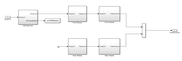
Figure : Tractive Force

The ‘Tractive force’ subsystem is as shown above.

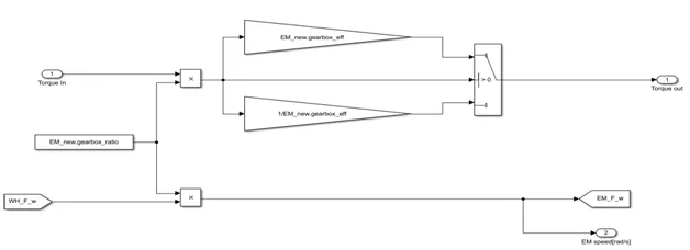
Figure : Gear Box

The output of the gear box depends upon the torque input from electric motor and the efficiency of the gear box.

The output of the gear box,

Torque out = Torque * Gear box ratio * Efficiency [For +ve Torque]

Torque out = Torque * Gear box ratio / Efficiency [For -ve Torque]

The electric motor speed, EM speed = Gear box ratio * wheel speed

The wheel speed (angular velocity) is calculated in front wheel model.

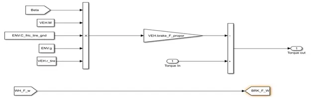
Figure : Front Brakes

The front brakes model is as shown above. The traction force in front wheels is provided by regenerative braking and mechanical braking.

The braking torque is given by,

Braking Torque = Brake signal * vehicle mass * ground friction * gravity * tire radius.

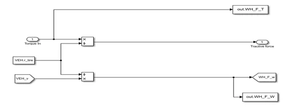
Figure : Front wheels

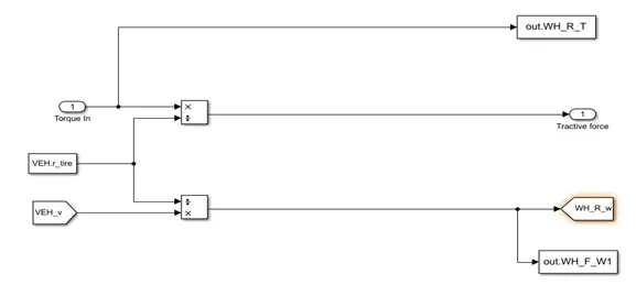
Figure : Rear Wheels

The front and rear wheels model is as shown above. The tractive force can be calculated as

Tractive force = Torque / radius of tire

The angular velocity of the vehicle calculated as

Angular velocity = Vehicle velocity / radius of tire

This is being fed to the gear box block to find the electric motor speed.

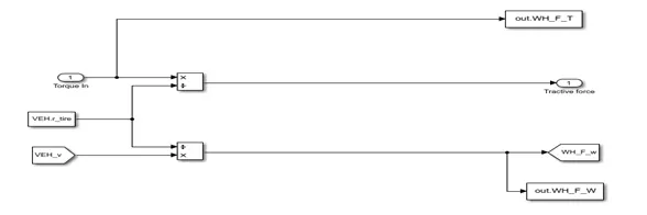
Figure : Rear Brakes

Only mechanical braking is applied to rear wheels. So the torque input is connected to ground. And the tractive force is calculated similarly as front brakes block in figure 11.

Since the Torque input is zero, there won ‘be any tractive force generated in this block shown in figure12.

3.2.4 Energy Management System

The Energy Management system should allow energy sources to operate in their optimum performance range and at the same time it should be able to provide power even if any sources are not available. Hybrid energy management system has the advantage of providing uninterruptible power in almost all cases.

In our case we are considering three energy sources for power distribution.

The operating range of each of the sources are as follows.

Back up power distribution is as follows.

Inside 'Positive power subsystem, Power has been comapred using interval test block and switches. The primary power distribution is as shown in table above.

Inside 'Positive power' subsystem, there is another subsystem called 'Backup_power'. Inside that the battery SOC and fuel cell SOC have considered and back up power options are provided for each condition as explained in table above.

Figure : Compressor_model subsystem

The air flow rate from the compressor depend on the following values.

1. Pressure ratio
2. Compressor speed
3. Adiabatic efficiency

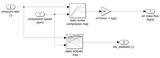
Figure : Static screw compressor map

The adiabatic efficiency map gives the efficiency of the compressor for different compressor speed and pressure speed.

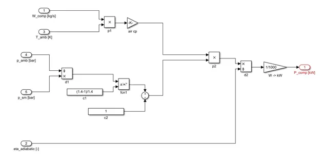
Figure : Power

The compressor output power can be calculated as follows[2] :

P_comp = (W_comp * T_amb * Cp) * (((P₂/P₁) ^(1.4-1/1.4) -1) / eta_adiabatic)

Where W_comp = air flow rate[kg/s]

T_amb – Ambient temperature

Cp - specific heat at constant pressure (J/gK)

P2 – Raised pressure

P1 – Atmospheric pressure

3.2.6 Battery model

The Li-Ion battery model is as shown in figure13. The input to the model is the power request from the EMS. There are two subsystems inside it.

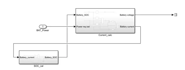
Figure : Battery model

1. Current_calc
2. SOC_cal

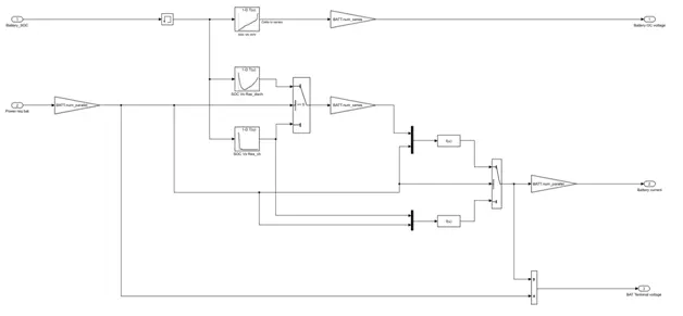
Figure : Current calc

The current calculation subsystem is as shown above. Battery voltage is determined from SOC[5]. The open circuit voltage with SOC data for a single cell will be available from the datasheet. It has to be multiplies with total number of cells in series to get the total voltage of the battery pack.

There are 3 plots used in this model to calculate the current. The open circuit voltage of the battery is determined from the SOC Vs OCV plot.

The internal resistance of the battery will be different while charging and discharging. This value can be obtained from SOC Vs Resistance for discharging and charging curves.

Then current, I = sqrt(Power /R_(chg/disch))

The battery terminal voltage = Battery power / current

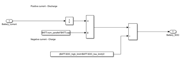
Figure : SOC

The SOC estimation of the battery is as shown above. There are various methods to estimate the SOC of a battery. The method adopted here is the coulomb counting method [5]. The Coulomb counting method measures the discharging current of a battery and integrates the discharging current over time in order to estimate SOC. Coulomb counting method is done to estimate the SOC(𝑡), which is estimated fromthe discharging current, 𝐼(𝑡), and previously estimated SOC values, SOC(𝑡 −1). SOC is calculated by the following equation[5]:

SOC(t) = SOC(t-1) + ( I(t) * Δt ) / Q_n

Where Q_n is the total Ah capacity of the battery. Here it is given as a constant value of 200Ah. Which is converted to mAh and fed to the block. There should be an initial SOC for the battery to provide emergency power to the vehicle. This is provided by another constant block.

Initial SOC = (Maximum SOC+ Minimum SOC) / 2

This SOC is fed to the current calculation block for current calculation. Since SOC is available after 1^st iteration, a memory block is added to avoid computational error.

3.2.7 Ultracapacitors

At the time of designing any system, primary source must be sized in such a manner that it can provide peak demand even though it occurs only for few seconds or minutes as compared to continues or average demand. Sizing whole system based on peak demand in place of average demand is very costly and inefficient as we are unable to utilize its full capacity all the time. But if we design system by storing electrical energy from primary source to some other energy storage device and then delivering that stored energy to the load in forms of burst of power in a controlled manner whenever peak demand occurs for a period of time ranging from fraction of seconds to several minutes, we can improve operation of system significantly.

Fuel cells have an operating range in which gives maximum efficiency. Operating outside this region reduces the efficiency and performance. So it cannot be used for supplying transient power.

Batteries have many limitations like low power density, poor low temperature performance, can’t be charged or discharged at high rate over many hundreds of thousands cycles, requires repeated replacements throughout the life of system.

Ultra capacitors provide simple and highly reliable solution to bridge the short term power mismatches between power available and power required. They have much higher power density, extremely longer cycle life, wide temperature range (-40 to +65 degree) but low energy density.

In our system Ultra capacitors are designed to handle power demand above 55kW.

3.2.7.1 Modeling of Ultracapacitor in SIMULINK

The ultra capacitor model is as shown in the figure below. There are two subsystems inside it to estimate current and SOC.

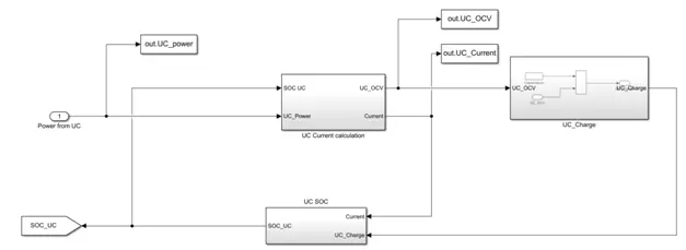
Figure : Ultra capacitor subsystem

There are three main blocks inside this subsystem.

1. UC Current calculation
2. UC SOC
3. UC Charge

Figure : UC Current calculation

The stored charge in an ultracapacitor is characterized by a normalized measure called the state of charge, SOC ∈ [0,1]. The state of charge of 0 represents no stored charge and 1 corresponds to full charge. The rate of change in ultracapacitor state of charge is proportional to the discharging or charging current I_cap (positive or negative values of current denote discharging or charging respectively)[4]:

d/dt (SOC(t) = (-1 / CVmax)* I_cap(t)

where C is the capacitance of the ultracapacitor module in Farads and Vmax is its voltage at full charge.

1. UC_Current
2. OCV
3. Charge on UC

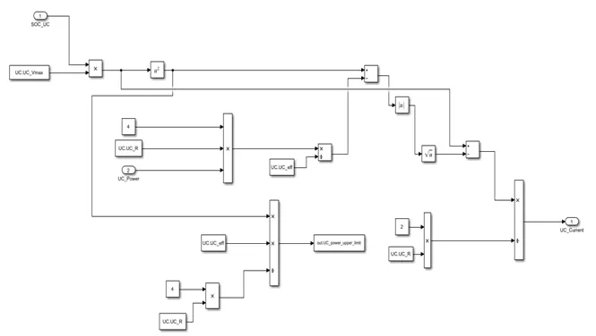
Figure : Current

The current of ultra capacitor can be calculated as given below[4].

I = SOC * V_max – sqrt (SOC * V_max ² – 4* R * PUC * eff

Where I = UC current

V_max = Maximum rated voltage at 100% SOC

R = lumped resistance

PUC = Power requested to ultra capacitor from EMS

Eff = Efficiency of ultra capacitor

Figure : OCV

The open circuit voltage of Ultra capacitor can be estimated as follows[4].

OCV =

This has been implemented above.

Unlike batteries UC doesn’t need complex SOC estimation methods. The SOC is proportional to Open circuit voltage.

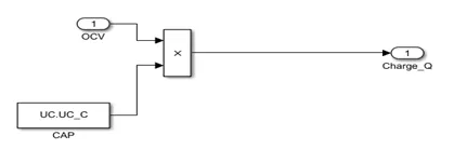
Figure : Charge on UC

The UC charge can be estimated by,

Charge, Q = OCV * C

Where C is the capacitance of UC.

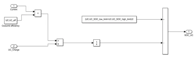
Figure : SOC

There should be an initial SOC for the battery to provide emergency power to the vehicle. This is provided by another constant block.

Initial SOC = (Maximum SOC+ Minimum SOC) / 2

The SOC of UC is given by,

SOC =

Where η= Charging efficiency of UC

As charging and the discharging of the ultracapacitor do not involve any chemical reaction they can be cycled with almost no deterioration. UC can withstand more than 1 million charge and discharge cycle. As the capacitance offered by UC is very high, energy density UC is also very high (10 times) compared to conventional capacitor and the power density is very high (10 times) compared to battery.

3.3Vehicle Model

There are certain resistances which are opposing vehicle movement. This includes rolling resistance of the tires, aerodynamic drag, and grading resistance. All these resistances are discussed below.

• Rolling Resistance (Fp)

The rolling resistance of tires on hard surfaces is primarily caused by hysteresis in the tire materials. This is due to the deflection of the carcass while the tire is rolling. The hysteresis causes an asymmetric distribution of ground reaction forces.

Rolling Resistance can be found as

Fp = M * g * u * cos (α)

Where u= rolling resistance coefficient

α= Grade angle

The rolling resistance coefficient, fr, is a function of the tire material, tire structure, tire temperature, tire inflation pressure, tread geometry, road roughness, road material, and the presence or absence of liquids on the road.

• Aerodynamic Drag (F_A)

A vehicle traveling at a particular speed in air encounters a force resisting its motion. This force is referred to as aerodynamic drag. It mainly results from two components: shape drag and skin friction.

Shape drag: The forward motion of the vehicle pushes the air in front of it. However, the air cannot instantaneously move out of the way and its pressure is thus increased, resulting in high air pressure.

Skin friction: Air close to the skin of the vehicle moves almost at the speed of the vehicle while air far from the vehicle remains still. The difference in speed between two air molecules produces a friction that results in the second component of aerodynamic drag.

Aerodynamic Drag

F_A = 1/2 * delta * A_f * C_d * V²

Where V= vehicle speed

A_f = vehicle frontal area

C_d = aerodynamic drag coefficient

Delta = air density

3.3.3 Grading Resistance (Fg)

When a vehicle goes up or down a slope, its weight produces a component and it is always directed to the downward direction. This component either opposes the forward motion (grade climbing) or helps the forward motion (grade descending). In vehicle performance analysis, only uphill operation is considered. This grading force is usually called grading resistance.

Grade Resistance

Fg = M * g * sin (alpha)

Where M = Mass of the vehicle

g= gravitational force

alpha = grading angle

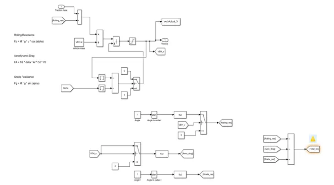
The above shown is the vehicle model. All the resistances mentioned above are implemented in this. The traction force should be more than all these resistances to keep the vehicle moving in forward direction.

The vehicle velocity is also calculated in this block.

Velocity =

Where Ft = Traction force

Fp = Rolling resistance

M = Mass of the vehicle

4. RESULT Analysis

The Actual velocity and desired velocity of the vehicle have been plotted in figure 33 and 34.

It has been understood that the vehicle designed here does not exactly follow the desired velocity. But it is somewhat similar in certain areas.

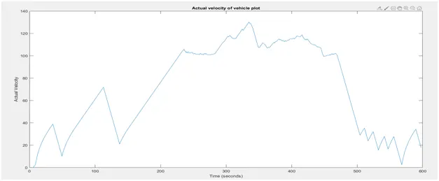
Figure : Actual velocity plot

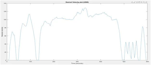
Figure : Torque request for power calculation

The torque request plot is shown above in figure 36. It can be observed that the torque is high for minimum speeds and less for maximum speeds.

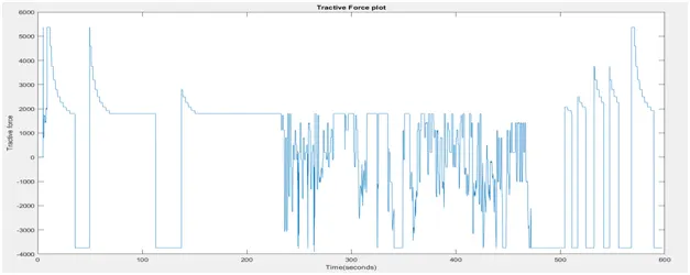
The Tractive force plot is shown in figure 37. It can be observed that Accelerating from o to maximum speed requires more tractive force and maintaining in a constant speed require less force.

4.2 Ultracapacitor output plots

The ultracapacitor open circuit voltage, current and power has been plotted in figures 41,42 and 43.

The OCV of ultra capacitor is proportional to State of charge. But here we have implemented only discharge circuits for UC. There is no charging circuit in this model. But we have given some amount of initial SOC so that it can deliver the desired power at all times. This is the reason in figure 41, the OCV does not drop below a certain voltage.

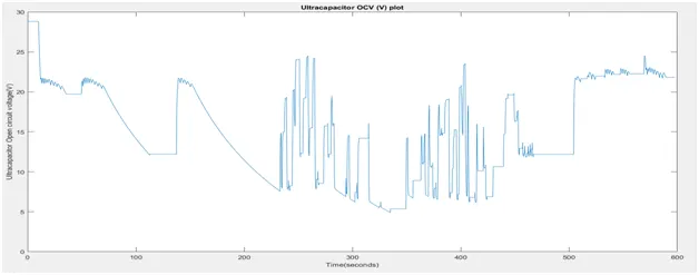
Figure : Ultracapacitor Open Circuit Voltage

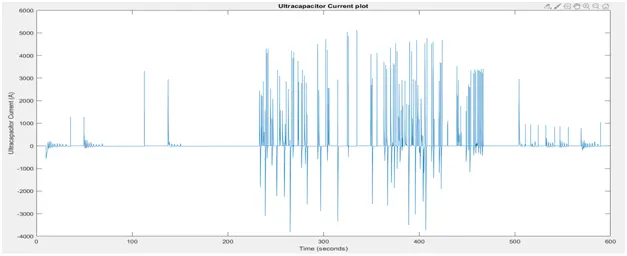
Figure : Ultracapacitor Current

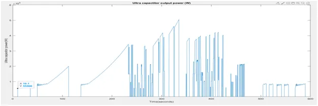
Figure : Ultracapacitor output power

For more accurate analysis we should implement charging circuit also. From the figure 42, we can understand that the current discharged by the ultra capacitor is very high during transient times. And it is un comparable with the current of fuel cell and battery. The Ultra capacitor output power is plotted in figure 43.

4.3 Battery Output plots

The Battery power, voltage, currents are plotted in figures 44,46 and 47. The battery is designed to operate below 23kW. It can be observed that the maximum battery voltage is 130V and maximum current is 175A.

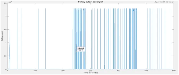
Figure : Battery Power

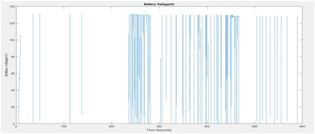
Figure : Battery Voltage

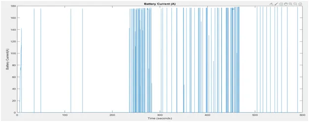
Figure : Battery Current

5. Conclusion

The complete model of Hybrid electric vehicle has been modelled and simulated using MATLAB Simulink. The following components were modelled successfully and analysed the output.

1. Driver model with acceleration and brake commands
2. Hybrid Electric power train which includes

• Controller
• Energy management for positive power with Fuel cell, Ultracapacitor and Battery
• Tractive force
• Fuel cell model
• Ultracapacitor model
• Battery model

3. Vehicle model