Genetic Algorithm using MATLAB
Aim:Genetic Algorithm using MATLAB
Genetic algorithms :
Genetic algorithms randomized search algorithms that have been developed in an effort to imitate the mechanics of natural selection and natural genetics. Genetic algorithms operate on string structures, like biological structures, which are evolving in time according to the rule of survival of the fittest by using a randomized yet structured information exchange
Stalagmite function:
stalagmite is an upward-growing mound of mineral deposits that have precipitated from water dripping onto the floor of a cave. Most stalagmites have rounded or flattened tips.
Syntax for genetic algorithm :
we can give the inputs by any one of the following ways-
Program:%input
x=linspace(0,0.6,150);
y=linspace(0,0.6,150);
num_spaces=50;
%forming 2d array
[xx,yy]=meshgrid(x,y);
for i=1:length(x)
for j=1:length(y)
input_vector(1)=xx(i,j);
input_vector(2)=yy(i,j);
f(i,j)=stagalmite(input_vector);
end
end
%study 1-unbounded
tic
for i=1:num_spaces
[results,fopt(i)]=ga(@stagalmite,2)
xopt(i)=results(1)
yopt(i)=results(2)
end
study_time1=toc
figure(1)
subplot(2,1,1)
surf(x,y,-f)
shading interp
hold on
plot3(xopt,yopt,-fopt,'marker','o')
subplot(2,1,2)
plot(-fopt)
xlabel('iteration')
ylabel('function maximum')
%study 2- bounded
tic
for i=1:num_spaces
[results,fopt(i)]=ga(@stagalmite,2,[],[],[],[],[0;0],[0.6;0.6])
xopt(i)=results(1)
yopt(i)=results(2)
end
study_time2=toc
figure(2)
subplot(2,1,1)
surf(x,y,-f)
shading interp
hold on
plot3(xopt,yopt,-fopt,'marker','o')
subplot(2,1,2)
plot(-fopt)
xlabel('iteration')
ylabel('function maximum')
%study3- increased initial population
tic
options=optimoptions('ga')
options=optimoptions(options,'populationsize',250)
for i=1:num_spaces
[results,fopt(i)]=ga(@stagalmite,2,[],[],[],[],[0;0],[0.6;0.6],[],[],options)
xopt(i)=results(1)
yopt(i)=results(2)
end
study_time3=toc
figure(3)
subplot(2,1,1)
surf(x,y,-f)
shading interp
hold on
plot3(xopt,yopt,-fopt,'marker','o')
subplot(2,1,2)
plot(-fopt)
xlabel('iteration')
ylabel('function maximum')
%stalagmite function code-
function A = stagalmite(input_vector)
x=input_vector(1);
y=input_vector(2);
f1=(sin(5.1*pi*x+0.5)).^6;
f2=exp((-4*log(2)*((x-0.0667).^2))/0.64);
f3=(sin(5.1*pi*y+0.5)).^6;
f4=exp((-4*log(2))*((y-0.0667).^2)/0.64);
A =-(f1*f2*f3*f4);
endcode explanation:
1.x=linspace(0,0.6,150);
y=linspace(0,0.6,150);
num_spaces=50
Initialise the values of x and y taking 150 values between the interval 0 and 0.6
2.function A = stalagmite(input_vector)
we use the genetic algorithm function to caluclate the maxima of the function.we store the outputs into results which contain maximas and fopt which contain the value at which the maxima is obtained.
3.[results,fopt(i)]=ga(@stagalmite,2)
xopt(i)=results(1)
yopt(i)=results(2)
end
study_time1=toc
figure(1)
subplot(2,1,1)
surf(x,y,-f)
shading interp
hold on
plot3(xopt,yopt,-fopt,'marker','o')
subplot(2,1,2)
plot(-fopt)
xlabel('iteration')
ylabel('function maximum')
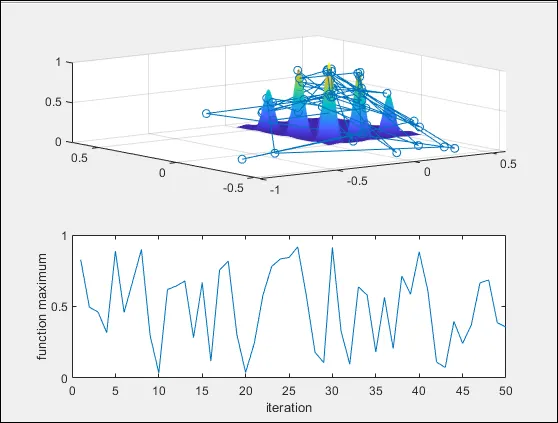
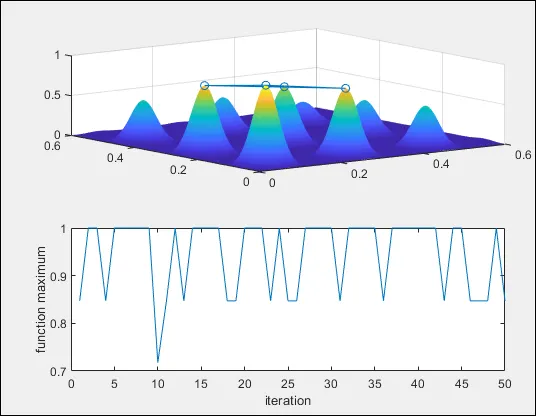
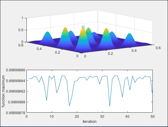
store the results into xopt, yopt.now we need to plot the surface of x,y,-f to get the 3D plot.We use the plot3 command to make a plot of xopt,yopt and -fopt to plot the optimum maximas.Also let us plot the fopt functio so that we can visualise the optimum values at each iteration. To get the time taken to complete cycle we used the tic toc commands to record the time.
Outputs and results:
Errors faced and solution to them:
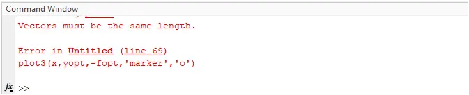
error of vectors of same lenghts at line no 69 plot3(x,yopt,-fopt,'marker','o') resolved by making the x as xopt and then go.