Project

AIM:-To prepare a technical report explaining the model properties & comments on the results.

Objectives:

Carry out a system-level simulation of an all-terrain vehicle and prepare a technical report explaining the model properties on the results.

All-Terrain Vehicle (ATV):-

An all-terrain vehicle (ATV) is defined as a motorized off-highway vehicle designed to travel on four low-pressure or non-pneumatic tires, having a seat designed to be straddled by the operator and handlebars for steering control.

STUDY #1:

CASE1:

SIMULINK MODEL FOR BAJA ATV WITH CVT

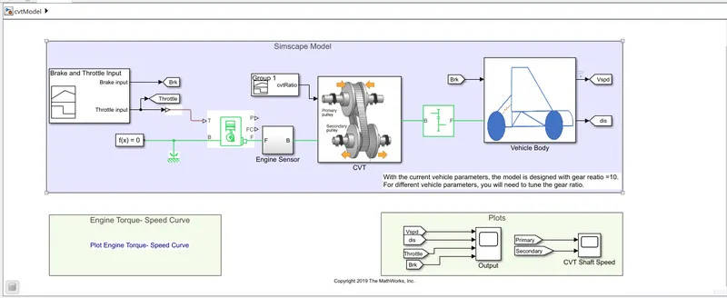
Major Components in this model:

• CVT
• Generic engine
• Vehicle body block

a)Continuously Variable Transmission drive (CVT):

It is better to have more gears in a transmission, since it can optimize engine speed in a variety of driving conditions. That means low gears can provide better acceleration while higher gears can maximize fuel economy. The majority of CVTs work via a pair of variable-diameter, cone-shaped pulleys connected by a steel or composite belt. The halves of each pulley are aligned with the pointed ends of the cones touching. These form a V-shaped groove in which the connecting belt rides. One side of the pulley is fixed, and the other side is movable, actuated by a hydraulic cylinder. The cylinder can increase or decrease the amount of space between the two sides of the pulley. This allows the belt to ride lower or higher along the walls of the pulley, depending on driving conditions, thereby changing the "gear" ratio.

CVT Block

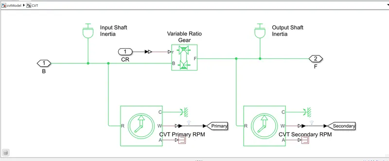
• Input shaft inertia represents the primary pully.
• Output shaft inertia represent the secondary pully.
• Variable gear ratio represent the variable gear box.

b)Generic Engine

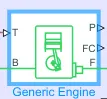
Represents a system-level model of spark-ignition and diesel engines suitable for use at initial stages of modelling when only the basic parameters are available. Optional idle speed and red line controllers are included. The throttle input signal T lies between zero and one and specifies the torque demanded from the engine as a fraction of the maximum possible torque.

Connections F and B are mechanical rotational conserving ports associated with the engine crankshaft and engine block, respectively. Connections P and FC are physical signal output ports through which engine power and fuel consumption rate are reported.

c)Vehicle body block

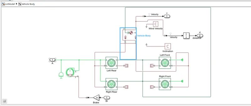
The Vehicle Body block represents a two-axle vehicle body in longitudinal motion. The vehicle can have the same or a different number of wheels on each axle. For example, two wheels on the front axle and one wheel on the rear axle. The vehicle wheels are assumed identical in size. The vehicle can also have a center of gravity (CG) that is at or below the plane of travel.

Graph of Input and Output of Case 1:

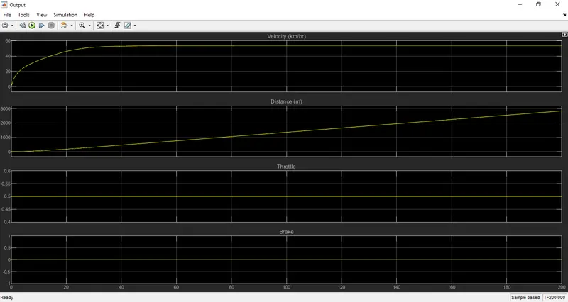
As we can see in above graph, the brake and throttle represent as input. The brake is constant at 0, means during entire simulation time brake is not applied. The throttle is also constant but at 0.5, means throttle is applied constantly without any fluctuation.

The Distance and Velocity represent output. The vehicle start at 0 distance at 0 sec, as time increase, distance increase slowly but exponentially till 40 sec after that distance increase linearly.

The velocity is is 0 Km/h at 0 sec, but as time increase the velocity shows logarithmic growth till 40 sec. At 40 sec, the velocity reaches at saturation velocity and then after velocity become constant approximately 55km/hr.

The Graph of CVT shaft speed.

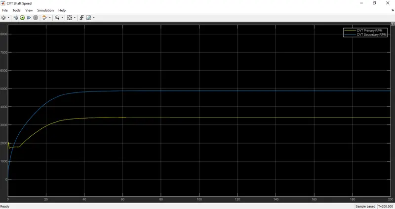
As we can see,primary shaft start at T=0 sec, the RPM reaches 2000 and then sudden fall in RPM and then increase lineraly till approximately T=10sec, after that increase logarithmically till 40 sec. The after the primary achieved rated RPM and rotate constantly at 3500 RPM.

Now, as we can see the graph of secondary shaft, at T=0 sec, the RPM is 0 and w.r.t time the RPM also increase logarithmitacally till T=40 sec. After that the secondary shaft also reached rated RPM or we can say, saturation RPM. After that Secondary shaft also revolves constantly at nearly 5000 RPM.

CASE2:

SIMULINK MODEL FOR BAJA ATV WITH CVT USING DASHBOARD:

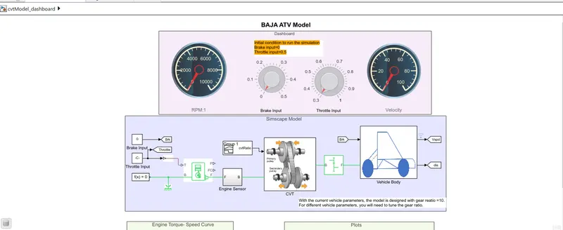
In this model we have a dashboard which contains knobs to control the inputs. A knob is provided to control both the parameters in real-time for the user.

The graph of Input and Output for Case 2

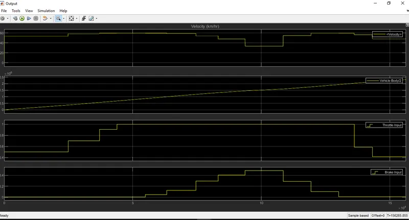
As we can see in above graph,When brake input is constantly zero, means brake is not applied and throttle input increase, the velocity also increases as per throttle input .When Throttle input is constant at particular value (throttle input should not be 0), and brake input is increase, means brake is applied, the velocity decrease as brake input. Means velocity decrease as brake input increase and velocity increase as brake input decrease.

The graph of CVT shaft speed of case 2:

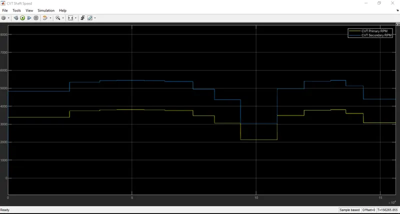
Here we can see,This graph indicates the variation in rpm of primary and secondary shafts with respect to input parameters. If RPM of Primary shaft is increase, the RPM of secondary shaft is also increase and if RPM of primary shaft is decrease, the RPM of secondary shaft is decrease. Means the RPM of Secondary shaft is increase or decrease as per RPM of primary shaft.

STUDY #2:

CASE 1:

SIMULINK MODEL FOR BAJA ATV WITH CVT USING LOOKUP TABLE:

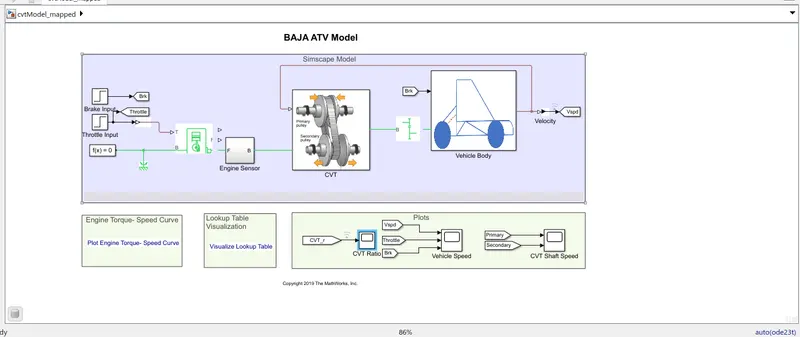
CVT Block:

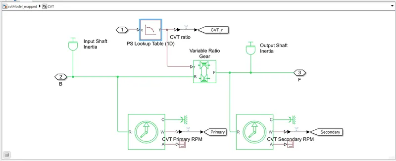
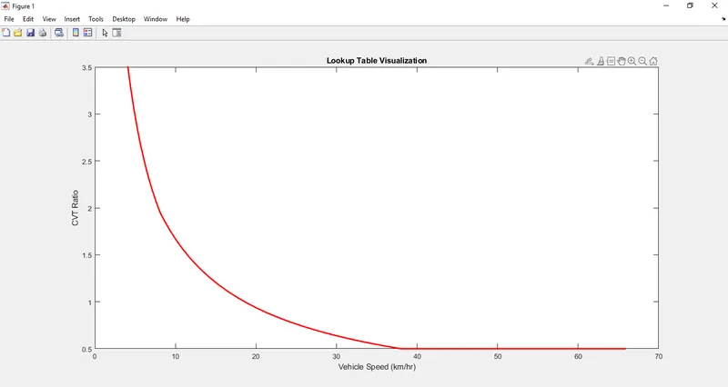
As we can see in above figure, The only Difference between this model and the first model is that in this model, the gear ratio input to CVT is provided using a lookup table.

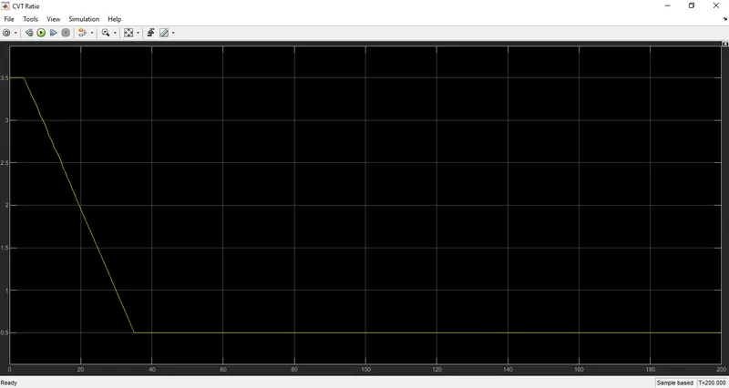
CVT Gear Ratio:-

Lookup table Visualisation:-

Output of 1st Case:-

Vehicle Speed:-

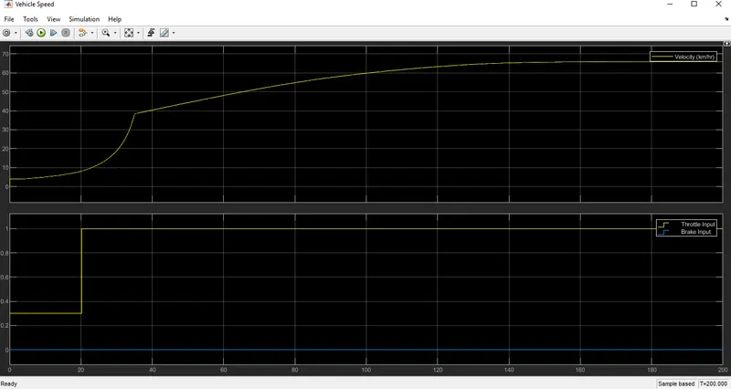
As we can see in above fig, the brake input is conatant at 0, means brake is not applied. The throttle input start at T=0sec and constant at 0.3 till T=20sec, in this time period the velocity reaches 5 to 10 kmph exponintially. At T=20, the throttle input increase 0.3 to 1 and then constant at 1 only till entite cycle period. Due to this throttle value velocity increase firstly exponentially then logarithmic.

CVT Shaft RPM:-

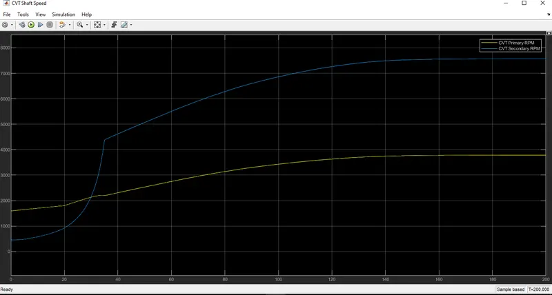
As we can see in above fig, the Rpm of primary shaft first increase linerly till T=20sec, then comparatively small logarathmic increament nearly T=35 sec, then increase logarathmically. Therefore as we can see, Secondary shaft also increase exponentially as per primary shaft till T=35 Sec, then increase logarathmically till run cycle.

STUDY #2:

CASE 2:

SIMULINK MODEL FOR BAJA ATV WITH CVT USING LOOKUP TABLE & DASHBOARD:

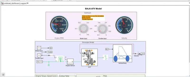
In this model a dashboard is used to control the inputs- ‘Throttle’ & ‘Brake’ with knobs.

Vehicle Speed:-

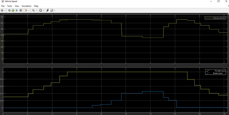
As we can see in above graph,When brake input is constantly zero, means brake is not applied and throttle input increase, the velocity also increases as per throttle input .When Throttle input is constant at particular value (throttle input should not be 0), and brake input is increase, means brake is applied, the velocity decrease as brake input. Means velocity decrease as brake input increase and velocity increase as brake input decrease. Here, Also same behavior in vehicle speed as per input of brake and throttle input.

So, We can the output of both the cases are same.

CVT RPM shaft:-

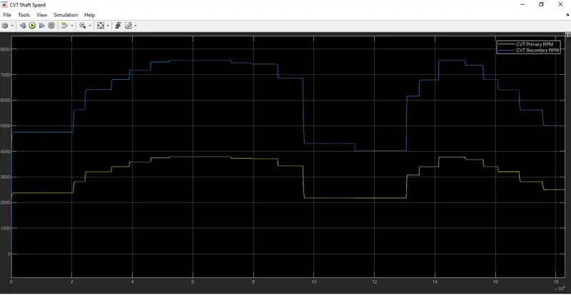
Here we can see, This graph indicates the variation in rpm of primary and secondary shafts with respect to input parameters. If RPM of Primary shaft is increase, the RPM of secondary shaft is also increase and if RPM of primary shaft is decrease, the RPM of secondary shaft is decrease. Means the RPM of Secondary shaft is increase or decrease as per RPM of primary shaft. So we can say in both the cases, CVT RPM shaft bahave similarly.

CONCLUSION:

Thus we have successfully analysed 4 different models of BAJA ATV WITH CVT and recorded the outputs: - (Vehicle velocity & CVT shaft rpm) with respect to variations in input throttle and brake.