Project 1 - Simulating a BTMS

AIM : The aim of this project is to simulate the flow through a BTMS model.

OBJECTIVES : The objectives of this project are as follows:

• Create an excel calculator to estimate the volumetric efficiency of a cell.
• Prove using analytical equations that material properties are relevant or irrelevant while performing seady state simulation.
• Run the simulations for different element length - 12 mm, 8 mm, 6 mm, 4 mm.
• Find out the element size which gives good accuracy using above objective results.

OBJECTIVE 1 :

EXCEL CALCULATOR

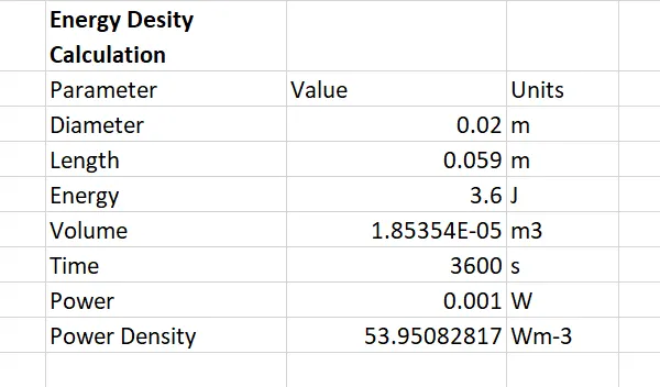
To find out the energy of the battery in Joules, firstly we need to know what will be the value of charge which is transferred and voltage of the battery at which the charge is transferred.

Charge can be expressed as 'Q' in unit 'Coloumb' .

Voltage can be expressed as 'V' in unit 'Volt' .

Charge and Voltage can be converted into energy using following equation:

Energy (J) = Charge (C) * Voltage (V)

E (J) = Q (C) * V (V)

And we can find out charge using below equation :

Charge (C) = Current (A) * time (s)

where Current is in Amperes (A)

Time is in seconds (s)

Firstly, we will calculate the energy for 1V battery transferring 1mA (milli Ampere) of current for 1 hour.

So, Q = 1e-3 (mA) * 3600 (s) = 3.6 C

and

E = 3.6 (C) * 1 (V) = 3.6 J

So, it is clear that for 1V battery which is transferring 1mA of current energy will be equal to 3.6J.

We can use these conversions to convert the voltage and charge of an electric vehicle battery and calculate the energy and the use the above excel calculator to figure out the Power density of the battery.

In the above example for 1V battery transferring 1mA current for 1 hour the power density is calculated to be 53.9508 W/m3.

OBJECTIVE 2 :

Experimentally, we can find out that the temperature variation depend on material property, as temperture in metals increases thermal conductivity (material property) decreases because with the increase in temperature the vibrations of molecules increases. So, the flow of free electrons is obstructed, thus reducing the conductivity.

Analytically we can prove by deriving 1D heat conduction equation that the temperature variation depends on the material.

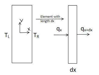
Consider an element in the solid of length dx with 1D conduction. Here we are assuming following things:

• The internal resistance in y direction is very low.
• The solid has very less thickness.

Using Energy Balance:

q(x) + H*V= q(x+dx)

where : q = heat supplied

dx = length of element

H = heat source generation per unt volume

using taylor eries expand above equation:

q(x) + H*Adx = q(x) + Δx(dq/dx) + (Δx^2/2!) * (d2q/dx2) + .....

Ignore H.O.T we get

q(x) + H*Adx = q(x) + Δx(dq/dx)

using fourier's law q = -kA(dT/dx) put value of q in dq/dx we get

-kA(d2T/dx2)dx = H(Adx)

d2T/dx2 = H/k

Above eqaution is the differential or governing equation for 1D heat conduction we can see that after integrating this equation and solving for constants using boundary conditions temperature variation will be inversly proportional to the thermal conductivity of the material so, we can say that the material is relevant while performng the steady sate solution.

OBJECTIVE 3 :

Firstly, I will setup the solid zone for each cell seperatly.

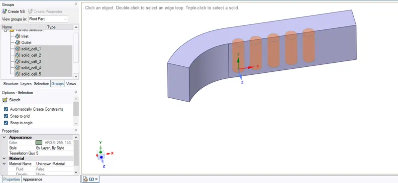
Now, I will try to run the smulations for different element length.

CASE 1 :

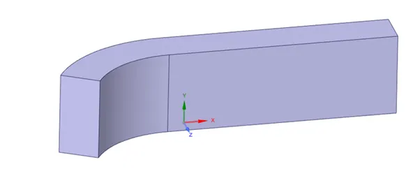
Geometry of BTMS model

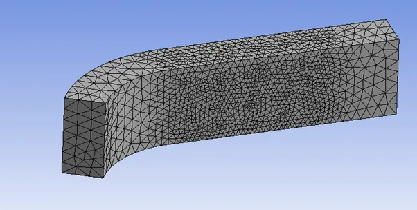
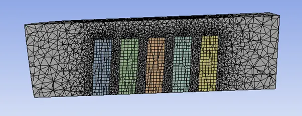
This CAD model contains 5 solid cells which will generate heat and the control volume of fluid is shown around the cell where the air will flow as a cooling fluid and the area where the calculations will be performed.

MESH OF THE CAD MODEL

The size of the element in above meshing is 12mm which leads to 85127 number elements for the whole geometry. In first screenshot it is visible that the tetrahedral is formed for the fluid control volume and for solid cell hexahedral mesh is generated, which can be seen in the section view in second screenshot.

Solver setup

• Solver Type - Density based solver
• State - Steady
• Model - Turbulence k-epsilon model
• Volumetric heat source - 30000 W/m3
• Inlet Boundary Condition (Velocity) - 4 ms-1
• Outlet Boundary Condition (Pressure) - 0 Pa

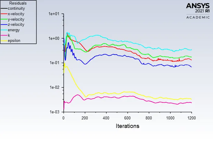
The simulation was run using above settings for 1200 iterations and the solutions was

converged on 1100 iterations.

Scaled Residual Plot

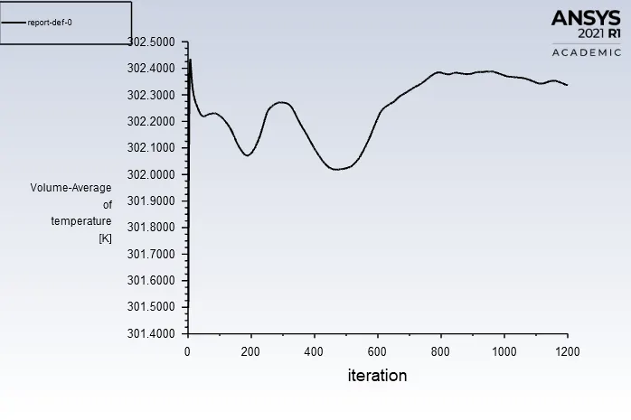
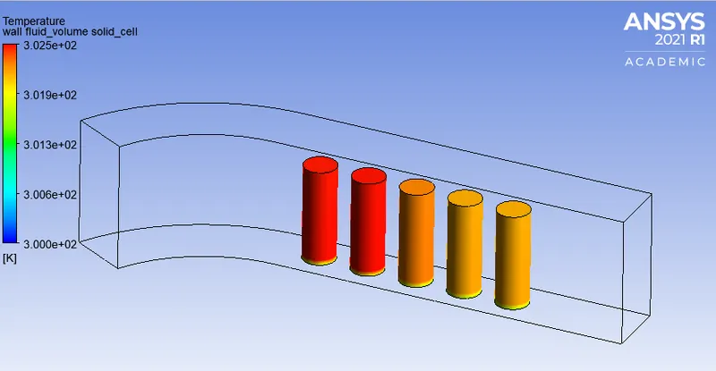
The value of the output temperature is 302.34K

Volume average Temperature Plot

Results

Temperature of Cells

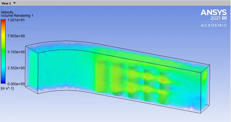
Volume Rendering of Velocity

CASE 2 :

Geometry of BTMS model

This CAD model contains 5 solid cells which will generate heat and the control volume of fluid is shown around the cell where the air will flow as a cooling fluid and the area where the calculations will be performed.

MESH OF THE CAD MODEL

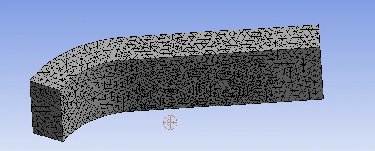
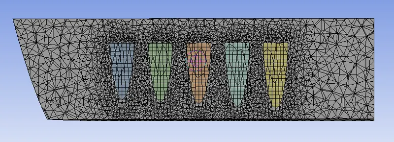
The size of the element in above meshing is 8mm which leads to 89135 number elements for the whole geometry. In first screenshot it is visible that the tetrahedral is formed for the fluid control volume and for solid cell hexahedral mesh is generated, can be seen in the section view in second screenshot.

Solver setup

• Solver Type - Density based solver
• State - Steady
• Model - Turbulence k-epsilon model
• Volumetric heat source - 30000 W/m3
• Inlet Boundary Condition (Velocity) - 4 ms-1
• Outlet Boundary Condition (Pressure) - 0 Pa

The simulation was run using above settings for 1200 iterations and the solutions was

converged on 1100 iterations.

Scaled Residual Plot

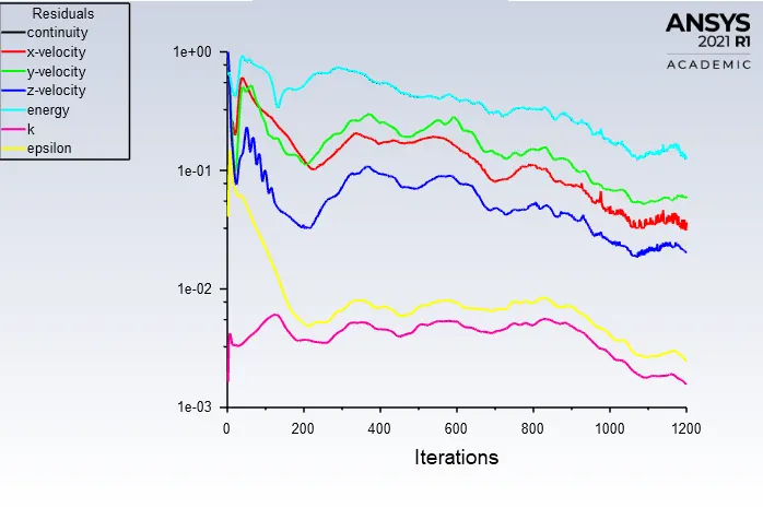
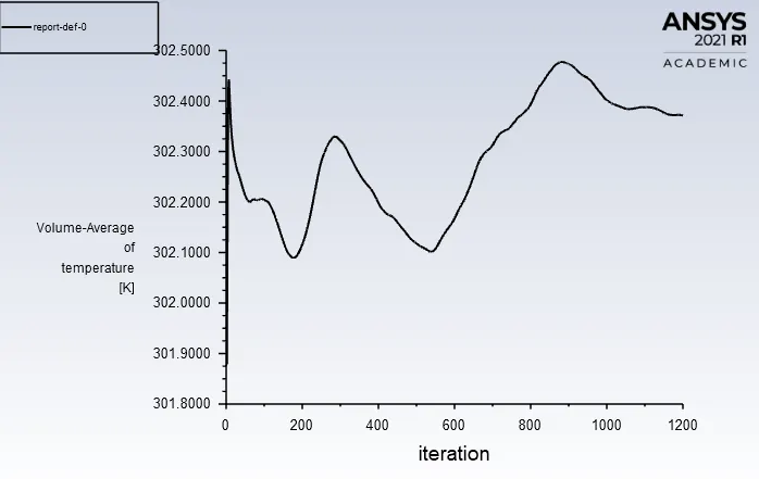
The value of the output temperature is 302.37K

Volume average Temperature Plot

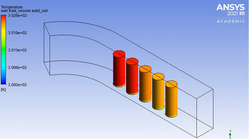
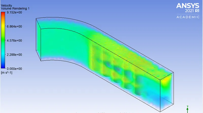
Results

Temperature of Cells

Volume Rendering of Velocity

CASE 3 :

Geometry of BTMS model

This CAD model contains 5 solid cells which will generate heat and the control volume of fluid is shown around the cell where the air will flow as a cooling fluid and the area where the calculations will be performed.

MESH OF THE CAD MODEL

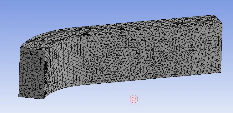
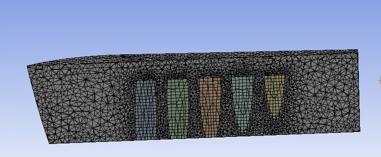
The size of the element in above meshing is 6mm which leads to 97327 number elements for the whole geometry. In first screenshot it is visible that the tetrahedral is formed for the fluid control volume and for solid cell hexahedral mesh is generated, can be seen in the section view in second screenshot.

Solver setup

• Solver Type - Density based solver
• State - Steady
• Model - Turbulence k-epsilon model
• Volumetric heat source - 30000 W/m3
• Inlet Boundary Condition (Velocity) - 4 ms-1
• Outlet Boundary Condition (Pressure) - 0 Pa

The simulation was run using above settings for 1200 iterations and the solutions was

converged on 1100 iterations.

Scaled Residual Plot

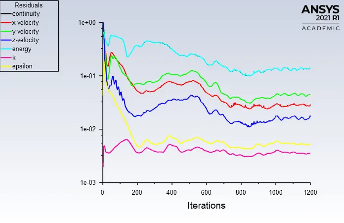
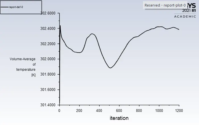
The value of the output temperature is 302.38K

Volume average Temperature Plot

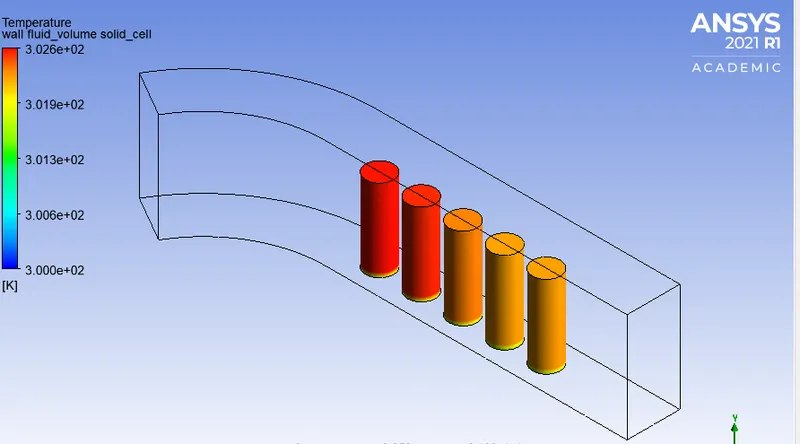
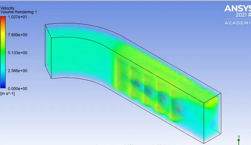
Results

Temperature of Cells

Volume Rendering of Velocity

CASE 4 :

Geometry of BTMS model

This CAD model contains 5 solid cells which will generate heat and the control volume of fluid is shown around the cell where the air will flow as a cooling fluid and the area where the calculations will be performed.

MESH OF THE CAD MODEL

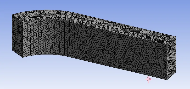
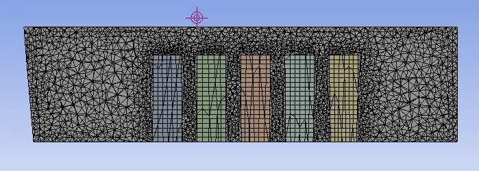
The size of the element in above meshing is 4mm which leads to 130746 number elements for the whole geometry. In first screenshot it is visible that the tetrahedral is formed for the fluid control volume and for solid cell hexahedral mesh is generated, can be seen in the section view in second screenshot.

Solver setup

• Solver Type - Density based solver
• State - Steady
• Model - Turbulence k-epsilon model
• Volumetric heat source - 30000 W/m3
• Inlet Boundary Condition (Velocity) - 4 ms-1
• Outlet Boundary Condition (Pressure) - 0 Pa

The simulation was run using above settings for 1200 iterations and the solutions was

converged on 1100 iterations.

Scaled Residual Plot

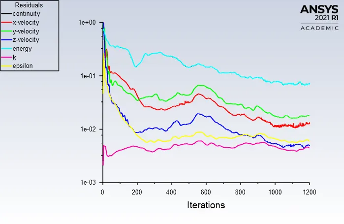
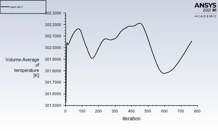
The value of the output temperature is 302.4K

Volume average Temperature Plot

Results

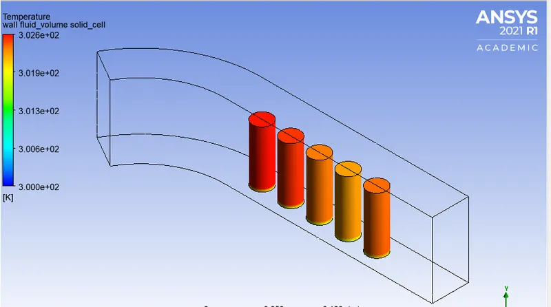
Temperature of Cells

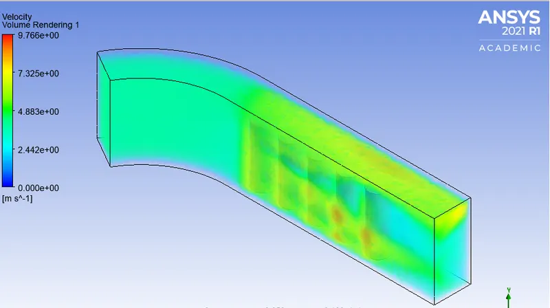
Volume Rendering of Velocity

OBJECTIVE 4 :

If we observe above results and output temperature we can see that the acurarcy of the solution is increasing by decreasing the element size but, only upto certain limit after that there is not much change in accuracy. We can observe that the output temperature after 6mm element size simulation (Case 3) doesn't change much by decreasing element size to 4mm.

CONCLUSION :

• The excel caculator to calculate power density is formed and how to measure energy of a cell with the help of equations is explained.
• The simulation of flow over 5 cells in a control volume is performed using air as a cooling fluid.
• Run the simulation for different element size and variation in the output result is observed.