Project-1: Powertrain for aircraft in runways
part A
1.ans
Aim: to Search and list out the total weight of various types of aircrafts.
Typical Airplane Weights
| Aircraft | Empty Weight | Max Fuel Weight | Max Cargo Weight | Max Gross Takeoff Weight |
|---|---|---|---|---|
| Antanov AN-225 | 628,000 lbs 285,000 kg |
661,400 lbs 300,000 kg |
417,000 lbs 190,000 kg |
1,411,000 lbs 640,000 kg |
| Airbus A380-800 | 611,000 lbs 277,000 kg |
560,000 lbs 254,000 kg |
185,000 lbs 84,000 kg |
1,268,000 lbs 575,000 kg |
| Boeing 747-800 | 485,300 lbs 220,100 kg |
427,400 lbs 194,000 kg |
295,000 lbs 134,000 kg |
987,000 lbs 447,700 kg |
| Airbus A340-500 | 370,000 lbs 168,000 kg |
386,300 lbs 175,000 kg |
119,000 lbs 54,000 kg |
820,000 lbs 372,000 kg |
| Boeing 777-300ER | 370,000 lbs 168,000 kg | 320,800 lbs 145,500 kg | 148,000 lbs 67,100 kg |
776,000 lbs 352,000 kg |
| Boeing 787-10 | 299,000 lbs 135,500 kg | 223,500 lbs 101,500 kg |
126,300 lbs 57,300 kg | 560,000 lbs 254,000 kg |
| Boeing 737-900 | 98,500 lbs 44,700 kg |
53,100 lbs 24,000 kg |
44,600 lbs 20,200 kg |
187,000 lbs 85,000 kg |
| Airbus A320-100 | 93,900 lbs 42,600 kg |
48,700 lbs 22,100 kg |
44,000 lbs 20,000 kg |
150,000 lbs 68,000 kg |
| Embraer 190 | 63,500 lbs 28,800 kg |
28,600 lbs 13,000 kg |
28,800 lbs 13,100 kg |
106,000 lbs 48,000 kg |
| Gulfstream G650 | 54,000 lbs 24,500 kg | 48,200 lbs 21,900 kg | 6,500 lbs 3,000 kg |
100,000 lbs 45,200 kg |
| Bombardier CRJ900 | 48,160 lbs 21,850 kg | 19,600 lbs 8,900 kg | 6,075 lbs 2,760 kg | 80,500 lbs 36,500 kg |
| Bombardier Q400 | 39,300 lbs 17,800 kg |
11,700 lbs 5,300 kg |
18,700 lbs 8,500 kg |
62,000 lbs 28,000 kg |
| Learjet 75 | 13,900 lbs 6,300 kg | 6,060 lbs 2,750 kg |
2,900 lbs 1,300 kg |
21,500 lbs 9,700 kg |
| Cessna Citation CJ4 | 10,300 lbs 4,700 kg | 5,800 lbs 2,650 kg |
2,200 lbs 1,000 kg | 17,200 lbs 7,800 kg |
| Beechcraft King Air B100 | 7,100 lbs 3,200 kg | 3,200 lbs 1,450 kg |
4,150 lbs 1,900 kg |
12,000 lbs 5,400 kg |
| Diamond DA50 RG | 3,200 lbs 1,450 kg |
340 lbs 155 lbs |
1,250 lbs 560 kg |
4,400 lbs 2,000 kg |
| Beechcraft Bonanza G36 | 2,500 lbs 1,150 kg | 450 lbs 200 kg |
850 lbs 385 kg |
3,660 lbs 1,660 kg |
| Cessna 206H | 2,200 lbs 990 kg |
520 lbs 235 kg |
1,150 lbs 520 kg |
3,600 lbs 1,630 kg |
| Sirrus SR22 | 2,250 lbs 1,000 kg | 485 lbs 220 kg |
950 lbs 430 kg |
3,600 lbs 1,630 kg |
| Cessna 172R | 1,700 lbs 770 kg |
380 lbs 170 kg |
560 lbs 255 kg |
2,425 lbs 1,100 kg |
MTOW = Maximum take-off weight,
MLW = Maximum landing weight,
TOR = Take-off run (SL, ISA+15°, MTOW),
LR = Landing run (SL, ISA+15°, MLW)
| Type | MTOW [kg] | MLW [tonnes] | TOR [m] | LR [m] | ICAO category | FAA category |
|---|---|---|---|---|---|---|
| Airbus A220-100 | 59,000 | 50.8 | 1,463 | 1,356 | Medium | Large |
| Airbus A220-300 | 65,000 | 57.61 | 1,890 | 1,494 | Medium | Large |
| Airbus A300-600[14] | 163,000 | 138 | 2,324 | 1,536 | Heavy | Heavy |
| Airbus A300-600R[14] | 192,000 | 140 | 2,385 | 1,555 | Heavy | Heavy |
| Airbus A310-200[14] | 142,000 | 123 | 1,860 | 1,480 | Heavy | Heavy |
| Airbus A310-300[14] | 157,000 | 124 | 2,290 | 1,490 | Heavy | Heavy |
| Airbus A318[18] | 59,000 | 57.5 | 1,375 | 1,340 | Medium | Large |
| Airbus A319[18] | 64,000 | 62.5 | 1,850 | 1,470 | Medium | Large |
| Airbus A320-100[18] | 68,000 | 66 | 1,955 | 1,490 | Medium | Large |
| Airbus A321-100[18] | 83,000 | 77.8 | 2,200 | 1,540 | Medium | Large |
| Airbus A330-200[12][13] | 242,000 | 180 | 2,220 | 1,750 | Heavy | Heavy |
| Airbus A330-300[12][13] | 242,000 | 185 | 2500 | 1750 | Heavy | Heavy |
| Airbus A330-900 | 251,000 | 191 | 3,100 | Heavy | Heavy | |
| Airbus A340-200[8][11] | 253,500 | 181 | 2990 | Heavy | Heavy | |
| Airbus A340-300[8][9] | 276,700 | 190 | 3000 | 1926 | Heavy | Heavy |
| Airbus A340-500[8] | 371,950 | 240 | 3,050 | 2,010 | Heavy | Heavy |
| Airbus A340-600[8] | 367,400 | 256 | 3,100 | 2,100 | Heavy | Heavy |
| Airbus A350-900 | 270,000 | 175 | 2,670 | 1,860 | Heavy | Heavy |
| Airbus A350-1000 | 308,000 | 233.5 | Heavy | Heavy | ||
| Airbus A380-800[1][2][3] | 575,000 | 394 | 3,100 | 1,930 | Heavy | Super |
| Airbus A400M | 141,000 | 122 | 980 | 770 | Heavy | Heavy |
| Antonov An-124-100M | 405,060 | 330 | 2,520 | 900 | Heavy | Heavy |
| Antonov An-225 | 640,000 | 591.7 | 3,500 | Heavy | Super | |
| ATR 42-500 | 18,600 | 18.3 | 1,165 | 1,126 | Medium | Small |
| ATR 72-600 | 22,800 | 22.35 | 1,333 | 914 | Medium | Large |
| Avro RJ-85 | 42,000 | 36.74 | Medium | Large | ||
| BAe Jetstream 41 | 10,890 | 10.57 | 1,493 | 826 | Medium | Small |
| Beechcraft 1900D | 7,765 | 7.605 | 1,036 | 853 | Medium | Small |
| Boeing 377 | 67,000 | Medium | Large | |||
| Boeing 707-120B[15] | 117,000 | 86.3 | Medium | Large | ||
| Boeing 707-320B[15] | 151,000 | 97.5 | Heavy | Heavy | ||
| Boeing 707-320C[15] | 151,000 | 112.1 | Heavy | Heavy | ||
| Boeing 717-200BGW | 50,000 | 46.265 | 1,950 | Medium | Large | |
| Boeing 717-200HGW | 55,000 | 47.174 | 1,950 | Medium | Large | |
| Boeing 720[16] | 104,000 | 79.5 | Medium | Large | ||
| Boeing 720B[16] | 106,000 | 79.5 | Medium | Large | ||
| Boeing 727-100[17] | 72,500 | 62.4 | Medium | Large | ||
| Boeing 727-100C[17] | 72,500 | 62.4 | Medium | Large | ||
| Boeing 727-200[17] | 78,000 | 68.1 | Medium | Large | ||
| Boeing 727-200 Advanced[17] | 84,000 | 70.1 | Medium | Large | ||
| Boeing 737-300 | 63,000 | 51.7 | 1,939 | 1,396 | Medium | Large |
| Boeing 737-400 | 68,000 | 54.9 | 2,540 | 1,540 | Medium | Large |
| Boeing 737-500 | 60,000 | 49.9 | 1,832 | 1,360 | Medium | Large |
| Boeing 737-600 | 66,000 | 54.66 | 1,796 | 1,340 | Medium | Large |
| Boeing 737-700 | 70,000 | 58.06 | 1,921 | 1,415 | Medium | Large |
| Boeing 737-800 | 79,000 | 65.32 | 2,308 | 1,634 | Medium | Large |
| Boeing 737-900 | 85,000 | 66.36 | 2,500 | 1,704 | Medium | Large |
| Boeing 737-900ER | 85,000 | 71.35 | 2,804 | 1,829 | Medium | Large |
| Boeing 747-8 | 443,613 | 306.175 | 3,100 | Heavy | Heavy | |
| Boeing 747-8F | 447,700 | 346.091 | 3,100 | 1,800 | Heavy | Heavy |
| Boeing 747-100[7] | 340,200 | 265.3 | Heavy | Heavy | ||
| Boeing 747-200[7] | 377,840 | 285.7 | 3,338 | 2,109 | Heavy | Heavy |
| Boeing 747-300[7] | 377,840 | 260.32 | 3,222 | 1,905 | Heavy | Heavy |
| Boeing 747-400 | 396,900 | 295.742 | 3,018 | 2,179 | Heavy | Heavy |
| Boeing 747-400ER | 412,770 | 295.742 | 3,090 | Heavy | Heavy | |
| Boeing 757-200 | 116,000 | 89.9 | 2,347 | 1,555 | Medium | Large |
| Boeing 757-300 | 124,000 | 101.6 | 2,550 | 1,750 | Medium | Large |
| Boeing 767-300 | 159,000 | 136.078 | 2,713 | 1,676 | Heavy | Heavy |
| Boeing 767-300ER | 187,000 | 136.08 | 2,713 | 1,676 | Heavy | Heavy |
| Boeing 767-400ER | 204,000 | 158.758 | 3,414 | Heavy | Heavy | |
| Boeing 777-200ER | 297,550 | 213 | 3,380 | 1,550 | Heavy | Heavy |
| Boeing 777-200LR | 347,450 | 223.168 | 3,000 | Heavy | Heavy | |
| Boeing 777-300 | 299,370 | 237.683 | 3,380 | Heavy | Heavy | |
| Boeing 777-300ER | 351,800 | 251.29 | 3,100 | Heavy | Heavy | |
| Boeing 777F | 347,800 | 260.816 | 2,830 | Heavy | Heavy | |
| Boeing 787-8[10] | 228,000 | 172.365 | 3,300 | 1,695 | Heavy | Heavy |
| Boeing 787-9[10] | 254,000 | 192.777 | 2,900 | Heavy | Heavy | |
| Boeing 787-10[10] | 254,000 | 201.849 | Heavy | Heavy | ||
| Bombardier CRJ200 | 23,000 | 21.319 | 1,918 | 1,479 | Medium | Large |
| Bombardier CRJ700 | 33,000 | 30.39 | 1,564 | 1,478 | Medium | Large |
| Bombardier CRJ900[21] | 36,500 | 33.345 | 1,778 | 1,596 | Medium | Large |
| Bombardier Q400 | 28,000 | 28.01 | 1,219 | 1,295 | Medium | Large |
| Caravelle III | 46,000 | Medium | Large | |||
| Cessna Citation CJ4[26] | 7,761 | 7.103 | 1039 | 896 | Medium | Small |
| Concorde | 185,000 | 111.1 | 3,440 | 2,220 | Heavy | Heavy |
| Convair 880 | 87,500 | Medium | Large | |||
| de Havilland Comet 1 | 50,000 | Medium | Large | |||
| de Havilland Comet 2 | 54,000 | Medium | Large | |||
| de Havilland Comet 3 | 68,000 | Medium | Large | |||
| de Havilland Comet 4 | 70,700 | Medium | Large | |||
| de Havilland Hercules | 7,000 | Medium | Small | |||
| Douglas DC-4 | 33,000 | Medium | Large | |||
| Douglas DC-6 | 44,000 | Medium | Large | |||
| Douglas DC-6A | 48,600 | Medium | Large | |||
| Douglas DC-6B | 48,500 | Medium | Large | |||
| Douglas DC-7 | 55,000 | Medium | Large | |||
| Douglas DC-8-32 | 140,000 | Heavy | Heavy | |||
| Douglas DC-8-51 | 125,000 | Medium | Large | |||
| Douglas DC-8-61 | 147,000 | Heavy | Heavy | |||
| Embraer 120 Brasilia | 11,500 | 11.25 | 1,560 | 1,380 | Medium | Small |
| Embraer 170[22] | 36,000 | 32.8 | 1,644 | 1,274 | Medium | Large |
| Embraer 175[20] | 37,500 | 32.8 | 2,244 | 1,304 | Medium | Large |
| Embraer 190[19] | 48,000 | 43 | 2,056 | 1,323 | Medium | Large |
| Embraer ERJ 145 | 22,000 | 19.3 | 2,270 | 1,380 | Medium | Large |
| Embraer Phenom 100 | 4,800 | 4.43 | 975 | 741 | Light | Small |
| Embraer Phenom 300[25] | 8,150 | 7.65 | 956 | 677 | Medium | Small |
| Fokker 100 | 46,000 | 39.95 | 1,621 | 1,350 | Medium | Large |
| Handley Page Hermes | 39,000 | Medium | Large | |||
| Hawker Siddeley Trident 2E | 65,000 | Medium | Large | |||
| Ilyushin IL-86 | 208,000 | 175 | Heavy | Heavy | ||
| Ilyushin IL-96-300 | 250,000 | 175 | 2,600 | 1,980 | Heavy | Heavy |
| Ilyushin Il-96M | 270,000 | 195.04 | 3,115 | 2,118 | Heavy | Heavy |
| Learjet 75[23] | 9,752 | 8.709 | 1,353 | 811 | Medium | Small |
| Lockheed C-5 Galaxy[4][5][6] | 381,000 | 288.417 | 2,530 | 1,494 | Heavy | Heavy |
| Lockheed L-1011-200 | 211,400 | Heavy | Heavy | |||
| Lockheed L-1011-500 | 231,300 | 166.92 | 2,636 | Heavy | Heavy | |
| McDonnell Douglas DC-10 | 256,280 | 183 | 2,990 | 1,890 | Heavy | Heavy |
| McDonnell Douglas MD-11 | 273,300 | 185 | 2,990 | 1,890 | Heavy | Heavy |
| McDonnell-Douglas MD-83 | 73,000 | 63.28 | Medium | Large | ||
| McDonnell-Douglas MD-90-30 | 71,000 | 64.41 | 2,165 | 1,520 | Medium | Large |
| Pilatus PC-24[24] | 8,300 | 7.665 | 893 | 724 | Medium | Small |
| Saab 340 | 13,150 | 12.930 | 1,300 | 1,030 | Medium | Small |
| Saab 2000 | 22,800 | 21.5 | 1,300 | Medium | Large | |
| Scaled Composites Model 351 Stratolaunch | 589,670 | 3,660 | Heavy | Super | ||
| Tupolev Tu-154M | 104,000 | 80 | Medium | Large | ||
| Tupolev Tu-204SM | 104,000 | 87.5 | 2,250 | Medium | Large | |
| Vickers VC10 | 152,000 | 151.9 | Heavy | Heavy | ||
| Vickers Viscount 800 | 30,400 | Medium |
Large |
Helicopters
MTOW = Maximum take-off weight
| Type | MTOW [pounds] | MTOW [kg] | Power output [kW] | Power to weight [W/kg] | Rotor diameter [m] |
|---|---|---|---|---|---|
| Mil Mi-12[27] | 231,485 | 105,000 | 19,200 | 182 | 2 x 35 |
| Mil Mi-26[28] | 123,459 | 56,000 | 17,000 | 343 | 1 x 32 |
| Sikorsky CH-53K | 88,000 | 39,916 | 16,200 | 405 | 1 x 24 |
| Sikorsky CH-53E[29] | 73,500 | 33,300 | 9,810 | 294 | 1 x 24 |
| Boeing CH-47D/F Chinook[30] | 50,000 | 22,680 | 7,058 | 311 | 2 x 18.3 |
| AgustaWestland AW101[31] | 34,392 | 14,600 | 4,698 | 321 | 1 x 18.59 |
| Sikorsky S-92[32] | 26,500 | 12,020 | 3,758 | 312 | 1 x 17.17 |
| Eurocopter EC225 Super Puma | 24,692 | 11,200 | 3,552 | 317 | 1 x 16.2 |
| Boeing Vertol CH-46 Sea Knight[33] | 24300 | 11,000 | 2,800 | 254 | 2 x 15.24 |
| NHIndustries NH90 | 23,370 | 10,600 | 3,324 | 314 | 1 x 16.3 |
| Eurocopter AS532 Cougar | 19,840 | 9,000 | 2,370 | 263 | 1 x 15.6 |
| Airbus Helicopters H160 | 13,340 | 6,050 | 1,910 | 316 | 1 x 13.4 |
| Bell 412EP | 1,1900 | 5,397 | 1,864 | 345 | 1 x 14.0 |
| Eurocopter EC145 C-2 | 7,903 | 3,585 | 1,100 | 307 | 1 x 11.0 |
| Eurocopter EC135 P2+/T2+ | 6,415 | 2,910 | 944 | 325 | 1 x 10.2 |
| Eurocopter EC635 P2 | 6,393 | 2,900 | 1,218 | 420 | 1 x 10.2 |
| AeroVelo Atlas (human powered) | 282 | 128 | 1.1 | 8.5 | 4 x 20.2 |
Convertiplanes
MTOW = Maximum take-off weight
| Type | MTOW [kg] | Power output [kW] | Power to weight [W/kg] | Rotor diameter [m] |
|---|---|---|---|---|
| Bell Boeing V-22 Osprey | 27,445 | 6,150 | 224 | 2 x 11.58 |
| Bell-Agusta BA609 | 7,600 | 1,447 | 190 | 2 x 7.92 |
| Bell XV-15 | 6,009 | 1,156 | 192 | 2 x 7.62 |
----------------xxxxxxxxxxxxxxxxxxxxxxx--------------------
2nd ans.
Ground Speed
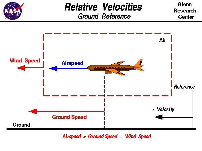
For a reference point picked on the ground, the aircraft moves relative to the reference point at the ground speed. Ground speed is also a vector quantity so a comparison of the ground speed to the wind speed must be done according to rules for vector comparisons.
Airspeed
The important quantity in the generation of lift is the relative velocity between the object and the air, which is called the airspeed. Airspeed cannot be directly measured from a ground position, but must be computed from the ground speed and the wind speed. Airspeed is the vector difference between the ground speed and the wind speed.
Airspeed = Ground Speed - Wind Speed
On a perfectly still day, the airspeed is equal to the ground speed. But if the wind is blowing in the same direction that the aircraft is moving, the airspeed will be less than the ground speed.
Examples
Suppose we had an airplane that could take off on a windless day at 100 mph (liftoff airspeed is 100 mph). We are at an airport with an east-west runway that is 1 mile long. The wind is blowing 20 mph towards the west and the airplane takes off going east. The wind is blowing towards the aircraft which we call a headwind. Since we have defined a positive velocity to be in the direction of the aircraft's motion, a headwind is a negative velocity. While the plane is sitting still on the runway, it has a ground speed of 0 and an airspeed of 20 mph:
Airspeed = Ground Speed (0) - Wind Speed (-20) = 20 mph
The airplane starts its take off roll and has a constant acceleration a. From Newton's second law of motion, the ground speed V at any time t is:
V = a * t
and the distance d down the runway at any time is:
d = 1/2 * a * t^2
For a fixed length runway, this specifies the time to be used in the velocity equation. Let's assume that at 5000 feet down the runway, the velocity is 80 mph. Then the airspeed is given by
Airspeed = Ground Speed (80) - Wind Speed (-20) = 100 mph
and the airplane begins to fly. Now another pilot, with exactly the same airplane decides to take off to the west. The wind is now in the same direction as the motion and this is called a tailwind. The sign on the wind speed is now positive, not negative as with the headwind. The acceleration along the ground is the same, so at 5000 feet down the runway, the ground speed is again 80 mph. The airspeed is then given by:
Airspeed = Ground Speed (80) - Wind Speed (20) = 60 mph
This airplane doesn't have enough airspeed to fly. It runs off the end of the runway!
------------------xxxxxxxxxxxxxxxxxx------------------
3rd ans.
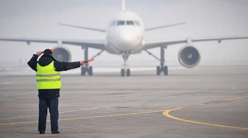
For movement on the ground the aircraft uses it own engine power, which is called taxing.
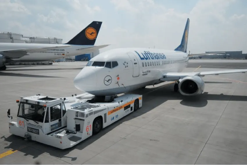
Although many aircrafts are capable of moving in backward using reverse thrust, as result the jet blast or prop wash might cause damage to the terminal building or equipment. Engine close to ground may also blow sand and debris forward and then suck them into the engine, causing damage to the engine. Therefore there are pushback trucks in the airport. A pushback truck lifts the front weel of the aircraft, their role in most airports is to move the aircraft away from the parking spot on to the taxiways, which is called towing.
Unwanted consequences mainly arising from the unintended movement of the aircraft during engine running.
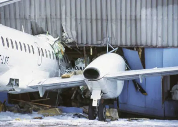
i) Effectively a loss of control can happen, especially during high power engine running. Damage can occur to the aircraft itself, other aircraft nearby or to airside structures.
ii) There is a risk of injury to ground support personnel who may be in relatively close proximity to the aircraft.
iii) It is easier for truck driver to see the surroundings better than the pilot sitting in the cockpit with limited window. The pushback driver knows the airport better than the pilot.
iv) It also saves fuel. virgin Atlantic had proposed a new system in which pushback truck will move the aircraft all the way to runway to save fuel and reduce impact of environment.
v) The plane engines are very loud. When more than one plane will add up their sound, than it will not be pleasent for passangers and others near airport.
-----------------------xxxxxxxxxxxxxxxxxxxx------------------
4th ans.
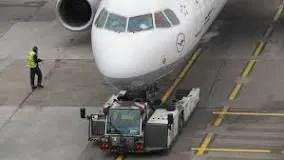
Pushback is when an aircraft is pushed backwards away from the airport gate by vehicles called tugs or tractors. Closer to departure, an aircraft tug will park right in front of the nose wheel. The tug might be directly attached to the plane's nose gear with a tow bar, or could be a "wheel-lift" tug.
Pushback is when an aircraft is pushed backwards away from the airport gate by vehicles called tugs or tractors.
Closer to departure, an aircraft tug will park right in front of the nose wheel.
The tug might be directly attached to the plane’s nose gear with a tow bar, or could be a “wheel-lift” tug. These tugs cradle the nose gear, then lift it up before moving the plane. That gives the tug driver control over the plane’s direction during pushback.
New taxi technologies are appearing, like pilot-controlled tugs, and electric motors mounted to the plane’s landing gear. Both promise to save fuel, and reduce airport noise.
------------xxxxxxxxxxxxxxxxxxx-------------------
5th ans.
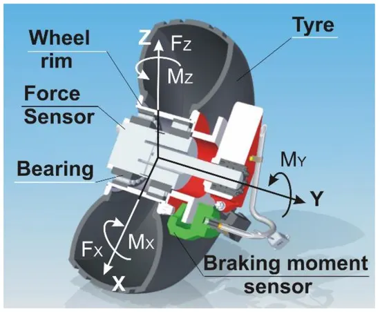
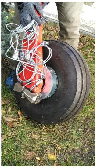
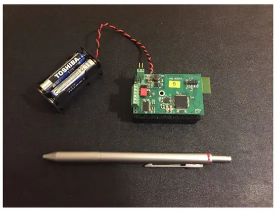
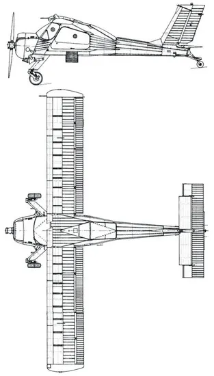
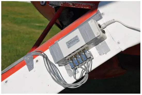
2.2. Airplane Used in the Experiment
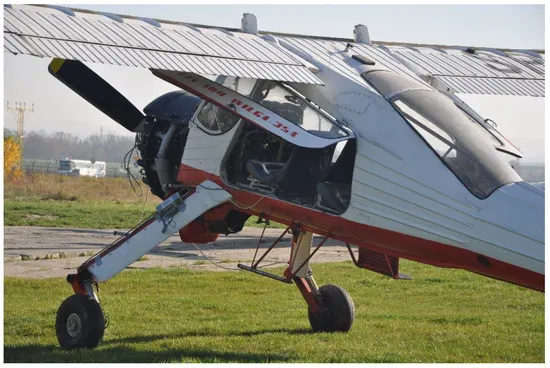
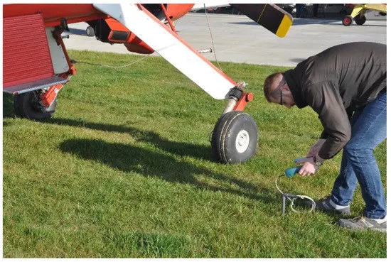
2.3. Grassy Airfield Conditions
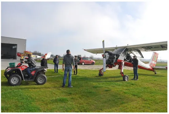
2.4. Field Procedures
-
Accelerating from stop to the taxi speed;
-
Taxiing with a constant speed (about 20–30 m);
-
Turning left or right;
-
Braking to a full stop or to block the wheels.
3. Results
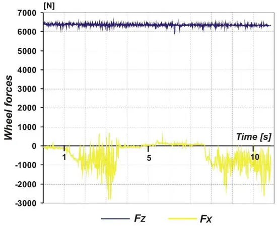
3.1. A General Presentation of the Results
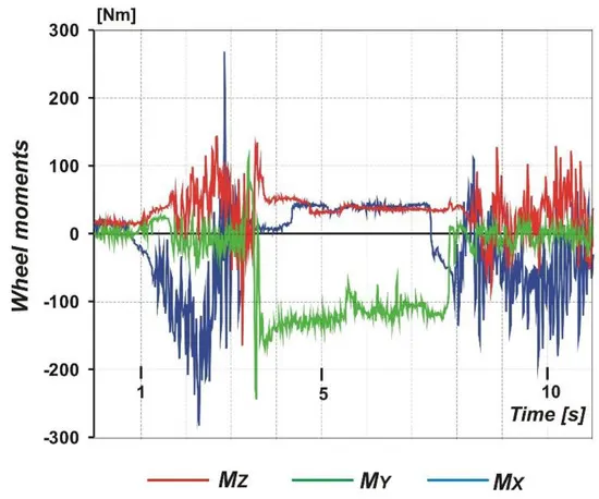
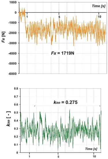
3.2. Rolling Resistance Coefficient
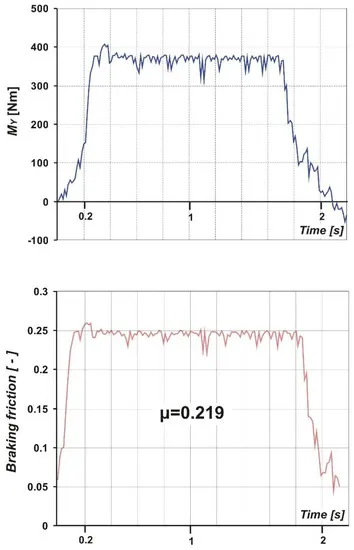
3.3. Braking Friction Coefficient
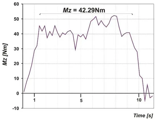
3.4. Aligning Moment
3.5. Effect of Weather Condidtions
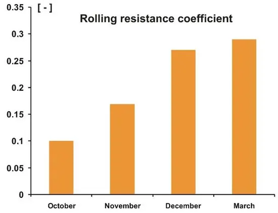
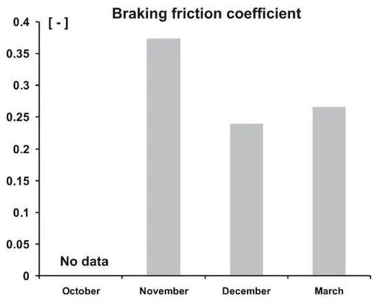
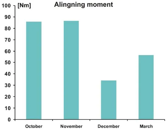
----------------------------------------xxxxxxxxxxxxxxxxxxxx-------------------------------------------
part B
6th ans
The force to move an airplane on an absolute flat runway with no wind at constant low speed is equal to the rolling resistance between the plane and the tarmac.
The rolling resistance for the air plane can be calculated as
Fr = c mr ag (1)
where
Fr = rolling resistance (N, lbf)
c = rolling resistance coefficient
mr = rolling mass (kg, lbm)
ag = acceleration of gravity (9.81 m/s2)
Example - Force required to pull an airplane at constant low speed on tarmac
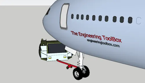
If the mass of a plane is 40000 kg and the rolling coefficient between the aircraft wheel and the tarmac is 0.02 - the force required to overcome the rolling resistance can be calculated as
Fr = 0.02 (40000 kg) (9.81 m/s2)
= 7848 N
This force can be delivered by a pulling truck or - as occasionally seen - by a number of pulling people. Enough weight for the pullers are required to create friction forces against the tarmac that equals the plane rolling resistance.
The friction force for the puller can be calculated to
Ff = μ W
= μ mf ag (2)
where
Ff = frictional force (N, lb)
μ = friction coefficient
W = weight (N, lbf)
mf = friction mass (kg)
Example - Required Mass for Pulling Truck
The friction coefficient between a pulling truck rubber wheels and dry tarmac is 0.9. Since pulling trucks are connected to air crafts nose wheels close to tarmac we simplify the calculation of required truck mass to
mf = (7848 N) / (0.9 (9.81 m/s2))
= 889 kg
Example - Air Craft Pulled by People
When persons participates in aircraft pulling there is normally an offset between the rope connected to the air craft nose wheel and the tarmac. It is common for persons to bend over with the rope over the shoulder or holding it in the hands.
The horizontal friction force between the persons shoes and the tarmac must be equal or larger than the air plane rolling resistance. The minimum required vertical force - or minimum weight of the people - depends on the bending angle as illustrated in the vector diagram below.
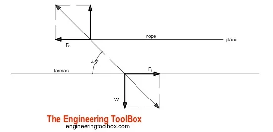
If they bend over 45o - the vertical force or weight equals to the horizontal force. With rubber shoes and the same friction coefficient as above for the truck the weight of the people should be 889 kg. With an average weight of 80 kg/person - the number of persons can be calculated to
n = (889 kg) / (80 kg/person)
= 11.1
= 12
With a more realistic bending angle 60o - the minimum vertical force or weight can be calculated as
W = tan(60o) (7848 N)
= 13593 N
The minimum mass of people to achieve this weight can be calculated as
mf = W / ag
= (13593 N) / (9.81 m/s2)
= 1386 kg
With an average weight of 80 kg/person - the minimum number of persons can be calculated to
n = (1386 kg) (80 kg/person)
= 17.3
= 18
other way of assumption
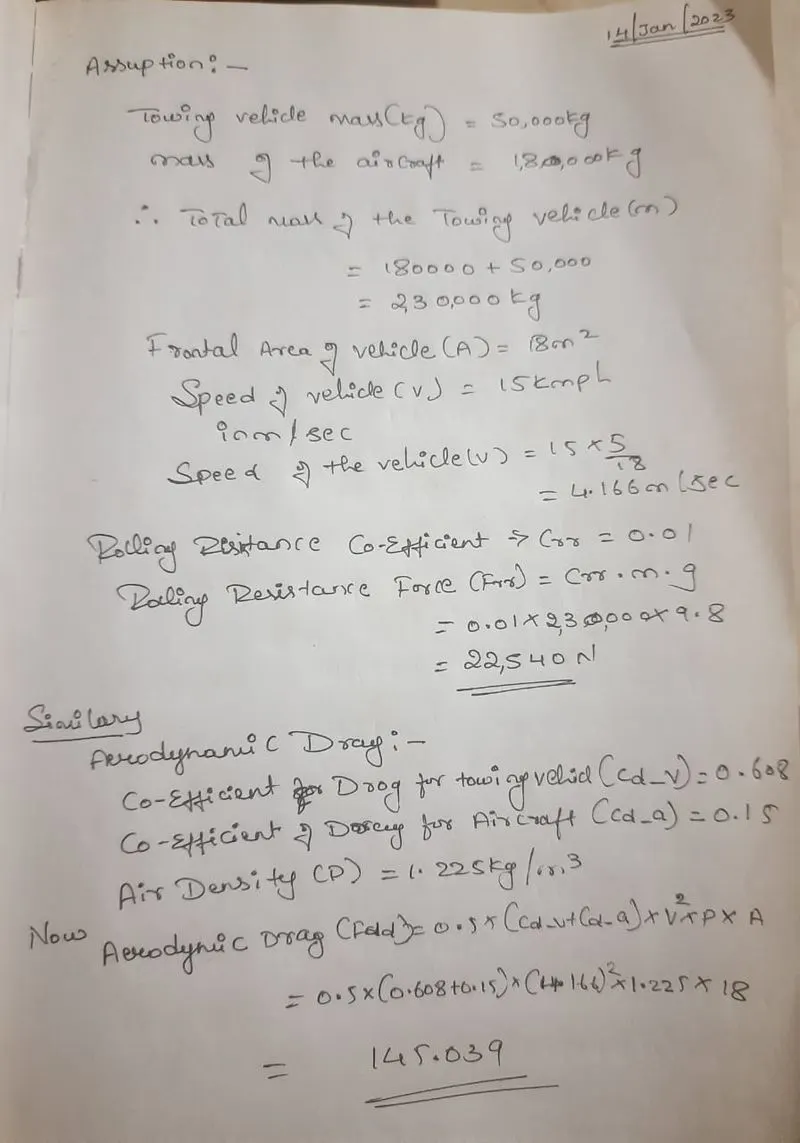
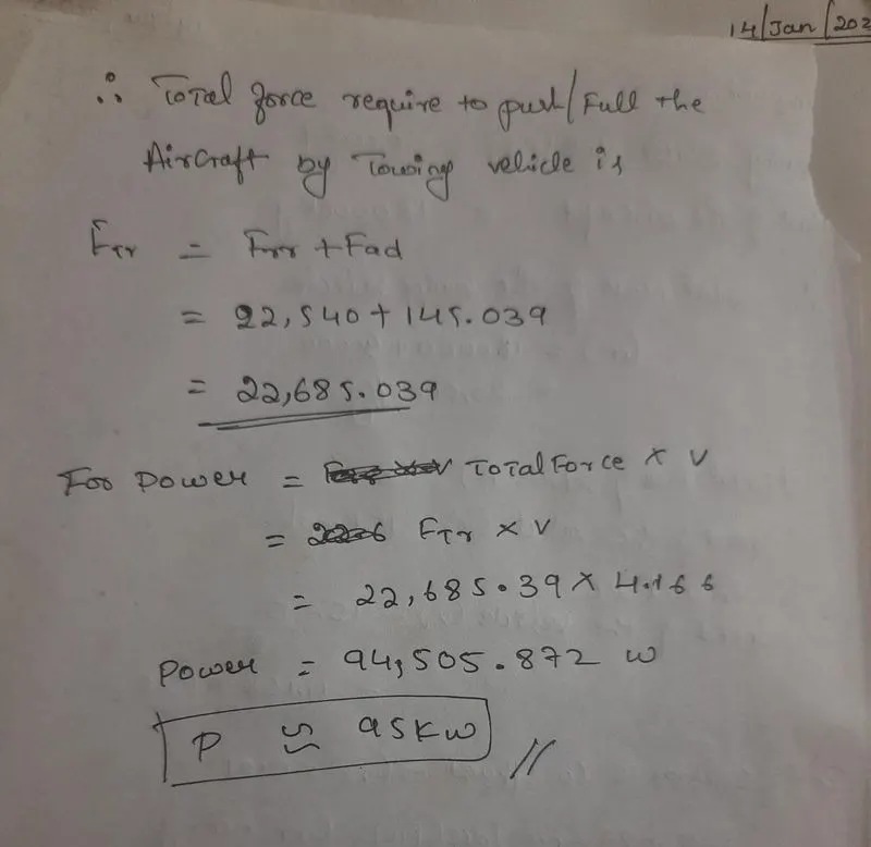
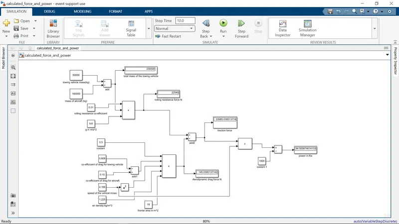
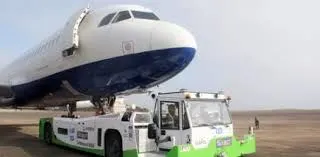
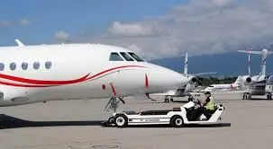
Figure shows the Towing Vehicle Application
| Assumation for Powertrain Design | |
| Parameter | Value |
| Aircraft Mass | 180000Kg |
| Towing Vehicle Mass | 50000 Kg |
| Rolling Resistance Co-efficient | 0.01 |
| Air Density | 1.225 Kg/m^3 |
| Towing Vehicle Drag Co-efficient | 0.608 |
| Aircraft Drag Co-efficient | 0.15 |
| Frontal Area | 18 m^2 |
| Inclination Angle | 0 rad |
| Tyre Pressure | 196 PSI/13.51 bar |
| Towing Velocity(V) | 15 Km/hr = 4.166m/s |
| Towing Time(t) | 2 min |
| Radius of the Towing Vehicle Wheel | 0.4 m |
Now from the above calculation we get the Total Force acting on the Vehicle as:
Total Traction Force(F) - 22685.039N
Power Required (P) - 94505.872 w = 95kw
Now, The Torque required by the vehicle to move is given by:
Torque(T) - Force(F)*Radius of the Wheel(R)
Therefore, T = 22685.039*0.4
= 9,0740.0156Nm
The Energy required by the vehicle for Towing application is given by:
Energy(E) = Power(P)*Towing Time
= 95*2/60
= 3.166kWh
For this application an electric motor which can be either a BLDC motor or an Induction Motor is choosen for the above power specs is given below:
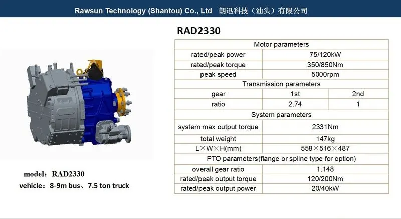
Here in the above figure, the Peak Motor Output Power given in the Motor Parameters in the input to the Towing Vehicle:
So therefore, Input Power to the Towing Vehicle(kW) - 120
Output Power of the Towing Vehicle(kw) - 95kW