Parsing NASA thermodynamic data and using the data in calculation
AIM:
To write a MATLAB program function to extract the 14 co-efficients, calculate the molecular weight, enthalpy, entropy and specific heat from the given data file.
GOVERNING EQUATIONS:
- Equation for Specific heat: `C_p / R = a_1+a_2T+a_3T^2+a_4T^3+a_5T^4`
- Equation for Enthalpy: `H/(RT) = a_1+(a_2T)/2+(a_3T^2)/3+(a_4T^3)/4+(a_5T^4)/5+a_6/T`
- Equation for Entropy: `S/R = a_1lnT+a_2T+(a_3T^2)/2+(a_4T^3)/3+(a_5T^4)/4+a_7`
OBJECTIVE:
The objective of the project is to learn to write data to & extract data from a file and use the data for other operations.
PROGRAMMING LANGUAGE:
MATLAB
CODE SAMPLE:
Main program:
%Program for parsing Thermodynamic data to/from a file
clear all
close all
clc

file = fopen('THERMO.dat','r'); %Opening the file THERMO.dat

line1 = fgetl(file); %reading the first line
line2 = fgetl(file); %reading the second line

A = strsplit(line2,' ');

global_low_temp = str2double(A{2});  %Calculating the Global low temperature
global_mid_temp = str2double(A{3});  %Calculating the Global mid temperature
global_high_temp = str2double(A{4});  %Calculating the Global high temperature

line3 = fgetl(file); %reading the third line
line4 = fgetl(file); %reading the fourth line
line5 = fgetl(file); %reading the fifth line

R = 8.3145;  %R - Universal Gas constant

for i = 1:53
B = fgetl(file);

%Getting the species name from the file
species_raw = B(1:6);

%Trimming the spaces from the species name
species = strtrim(species_raw);

%Creating sub-folders for each species
mkdir(species);

%Calculating the local low, mid & high temperatures
local_low_temp = str2double(B(46:55));
local_high_temp = str2double(B(58:64));
local_mid_temp =str2double(B(67:74));

B = fgetl(file);

c01 = str2double(B(1:15)); %Extracting Co-efficient 1
c02 = str2double(B(16:30)); %Extracting Co-efficient 2
c03 = str2double(B(31:45)) ;%Extracting Co-efficient 3
c04 = str2double(B(46:60)); %Extracting Co-efficient 4
c05 = str2double(B(61:75)); %Extracting Co-efficient 5

B = fgetl(file);

c06 = str2double(B(1:15)) ;%Extracting Co-efficient 6
c07 = str2double(B(16:30)); %Extracting Co-efficient 7
c08 = str2double(B(31:45)); %Extracting Co-efficient 8
c09 = str2double(B(46:60)); %Extracting Co-efficient 9
c10 = str2double(B(61:75)); %Extracting Co-efficient 10

B = fgetl(file);

c11 = str2double(B(1:15)); %Extracting Co-efficient 11
c12 = str2double(B(16:30)); %Extracting Co-efficient 12
c13 = str2double(B(31:45)); %Extracting Co-efficient 13
c14 = str2double(B(46:60)); %Extracting Co-efficient 14

temp = linspace(local_low_temp,local_high_temp,500); %Creating range of temperature values

%Naming the elements
elements = ['H','C','N','O','S','A'];

%Molecular weight is initially 0
mol_wt = 0;

%Feeding in the atomic weights of the elements
at_wt = [1,12,14,16,32,39.95];

for i=1:length(species)
for j =1:length(elements)

if strcmpi(species(i),elements(j))
mol_wt = mol_wt + at_wt(j);
position = j;

end
end

n = str2double(species(i));

if n>1
    mol_wt = mol_wt + at_wt(position)*(n-1);
end
end

%Displaying the molecular weight in the command window
fprintf('Molecular weight of %s %f n',species,mol_wt)
for i = 1:length(temp)

if temp(i) > local_mid_temp

%Calculating Specific heat (CP)
Cp(i) = calc_Cp(c01,c02,c03,c04,c05,c08,c09,c10,c11,c12,i,temp,R,local_mid_temp);

%Calculating Enthalpy (H)
H(i) = calc_H(c01,c02,c03,c04,c05,c06,c08,c09,c10,c11,c12,c13,i,temp,R,local_mid_temp);

%Calculating Entropy (S)
S(i) = calc_S(c01,c02,c03,c04,c05,c07,c08,c09,c10,c11,c12,c14,i,temp,R,local_mid_temp);

else

%Calculating Specific heat (CP)
Cp(i) = calc_Cp(c01,c02,c03,c04,c05,c08,c09,c10,c11,c12,i,temp,R,local_mid_temp);

%Calculating Enthalpy (H)
H(i) = calc_H(c01,c02,c03,c04,c05,c06,c08,c09,c10,c11,c12,c13,i,temp,R,local_mid_temp);

%Calculating Entropy (S)
S(i) = calc_S(c01,c02,c03,c04,c05,c07,c08,c09,c10,c11,c12,c14,i,temp,R,local_mid_temp);

end
end

%Plotting the Temperature vs Specific heat graph
figure(1)
plot(temp(1:i),Cp,'linewidth',2)

%Naming the x & y axis
xlabel('Temperature →')
ylabel('Specific heat →')

%Giving title for the graph
title('T vs Cp for',species)

%Saving the graph
saveas(figure(1),[pwd,'',species,'T vs Cp.png'])

%Plotting the Temperature vs Enthalpy graph
figure(2)
plot(temp(1:i),H,'linewidth',2)

%Naming the x & y axis
xlabel('Temperature →')
ylabel('Enthalpy →')

%Giving title for the graph
title('T vs H for',species)

%Saving the graph
saveas(figure(2),[pwd,'',species,'T vs H.png'])

%Plotting the Temperature vs Entropy graph
figure(3)
plot(temp(1:i),S,'linewidth',2)

%Naming the x & y axis
xlabel('Temperature →')
ylabel('Entropy →')

%Giving title for the graph
title('T vs S for',species)

%Saving the graph
saveas(figure(3),[pwd,'',species,'T vs S.png'])

end

%Closing the file
fclose(file);
Function to calculate Specific heat(Cp):
%Function to calculate the Specific heat
function [Cp] = calc_Cp(c01,c02,c03,c04,c05,c08,c09,c10,c11,c12,i,temp,R,local_mid_temp)

%If else to choose between high temperature & low temperature co-efficients
if temp(i)> local_mid_temp
Cp = R * (c01+(c02*temp(i))+((c03*(temp(i)).^2))+((c04*(temp(i)).^3))+((c05*(temp(i)).^4)));

else
Cp = R * (c08+(c09*temp(i))+((c10*(temp(i)).^2))+((c11*(temp(i)).^3))+((c12*(temp(i).^4))));

end %Ending the function
Function to calculate Enthalpy(H):
%Function to calculate the Enthalpy
function [H] = calc_H(c01,c02,c03,c04,c05,c06,c08,c09,c10,c11,c12,c13,i,temp,R,local_mid_temp)

%If else to choose between high temperature & low temperature co-efficients
if temp(i)> local_mid_temp
H = temp(i) * R * (c01 +((c02*temp(i))/2)+((c03*(temp(i))^2)/3)+((c04*(temp(i))^3)/4)+((c05*(temp(i))^4)/5)+(c06/temp(i)));

else
H = temp(i) * R * (c08 +((c09*temp(i))/2)+((c10*(temp(i))^2)/3)+((c11*(temp(i))^3)/4)+((c12*(temp(i))^4)/5)+(c13/temp(i)));

end %Ending the function
Function to calculate Entropy(S):
%Function to calculate the Entropy
function [S] = calc_S(c01,c02,c03,c04,c05,c07,c08,c09,c10,c11,c12,c14,i,temp,R,local_mid_temp)

%If else to choose between high temperature & low temperature co-efficients
if temp(i)> local_mid_temp
S = R * (c01*(log(temp(i)))+(c02*temp(i))+((c03*(temp(i))^2)/2)+(((c04*(temp(i))^3))/3)+((c05*(temp(i))^4)/4)+c07);

else
S = R * (c08*(log(temp(i)))+(c09*temp(i))+((c10*(temp(i)).^2)/2)+(((c11*(temp(i)).^3))/3)+((c12*(temp(i)).^4)/4)+c14);

end %Ending the function
ALGORITHM:
First, the file is opened and the data in the file is read line by line. As the data is read line by line, the global low, mid and high temperatures are read and stored in different variables. Each of the species are found and separated by assigning a separate variable for each of them. Then the local low, mid and high temperatures are read and separated. After that, the 14 co-efficients are separated. Then the Specific heat, Enthalpy & Entropy are calculated for a range of temperature values within the local low & high for that species. The molecular weight for the species is calculated and displayed in the command window. Then the calculation of Specific heat, Enthalpy & Entropy is done. It is done with the help of functions. After calculation, the values are plot on a graph against the temperature values. These plots are saved into separate folders for each of the species.
EXPLANATION:
The fopen command is used to open the file THERMO.dat. Along with the name of the file, an argument r is given to read the file. In case of writing data to the file, w is given as the argument. The THERMO.dat file is stored in the file id ‘file’. Next, the line 1 & 2 in the file is read using the fgetl command. They are stored in variables line 1 and line 2. In the second line, we have the global low, mid and high temperatures for the system. We use the strsplit command to split a character or string with a delimiter and extract the temperatures from the line of data. Then the next 3 lines are comments. They are skipped by using the fgetl command. Then we start a for loop to extract the name of the species, 14 co-efficients, calculate the Enthalpy, Entropy & Specific heat for all the species and plot graphs with the respective temperature values.
First, the species are extracted out from the line of data. The extracted species is then trimmed for leading & trailing spaces. Then the local low, mid and high temperatures are extracted for each species using the str2num or str2double command. Next, the coefficients are extracted from each line by fetching the data line by line and storing it in a variable B. From B, the co-efficient is extracted using the str2num or str2double command. This way, all the 14 co-efficients are extracted. After that, a range of the temperature values is created varying from the local low and local high temperatures. This is done using the linspace command. This range is stored in a variable temp. After this the elements that form the species and their atomic weights are given. With this the molecular weight of the species is calculated. It is done with the help of 2 for loops with loop counter variables i & j. Once the molecular weight is calculated, it is displayed in the command window using the fprintf command.
Then specific heat, enthalpy & entropy are calculated. When the high temperatures are taken, the high temperature co-efficients are used and when the low temperatures are taken, the low temperature co-efficients are used. To differentiate this, we use an if else command. The calculation of these values is done with the help of functions. This way, the Enthalpy, Entropy & Specific heat are calculated for all the temperature values in the temperature range. After that, the graphs are plot with the calculated values against the temperature values. Each graphs are plot in separate figure windows. The names for x & y axis and the title of the graphs is given using the xlabel, ylabel and title command. The plots are saved into the sub-folders with the species names with the help of saveas command.
RESULTS:
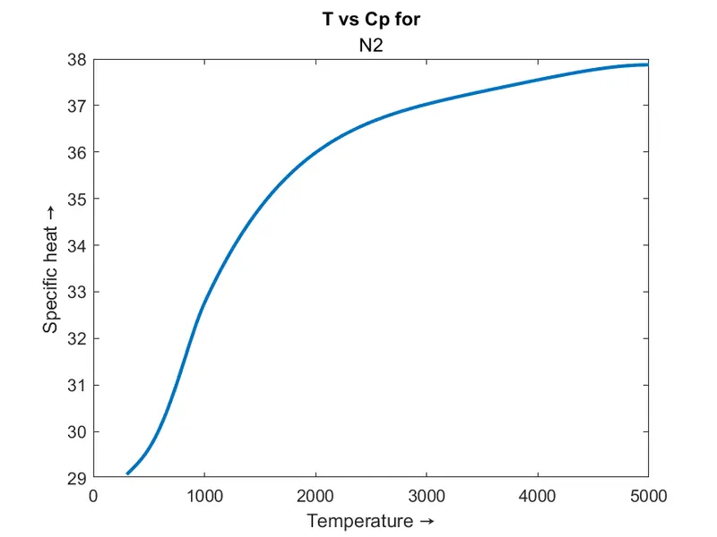
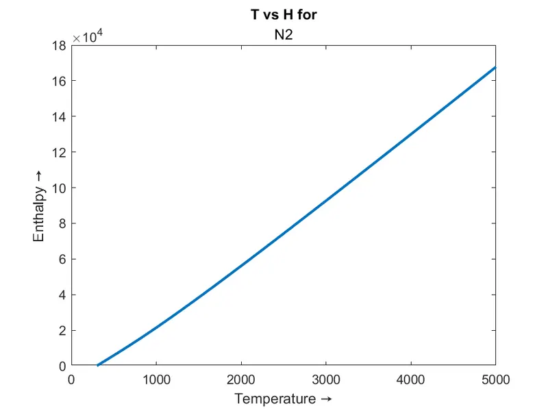
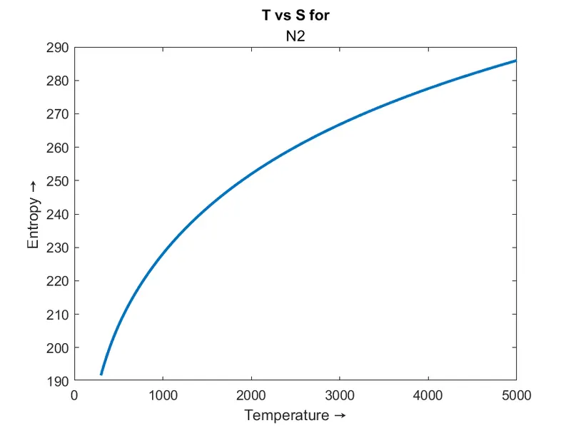
Plots of N2
These are the plots obtained for T vs Cp, T vs H and T vs S for the species N2 .
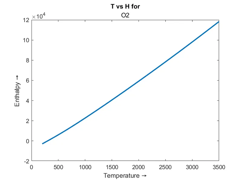
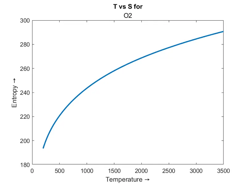
Plots of O2
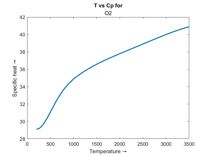
These are the plots obtained for T vs Cp, T vs H and T vs S for the species O2.
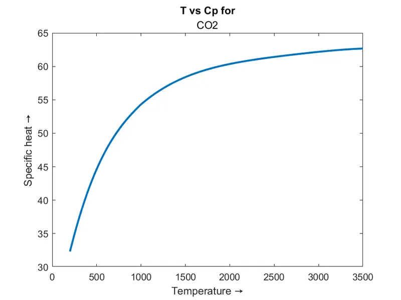
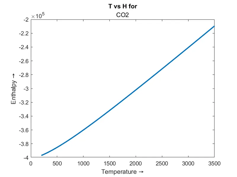
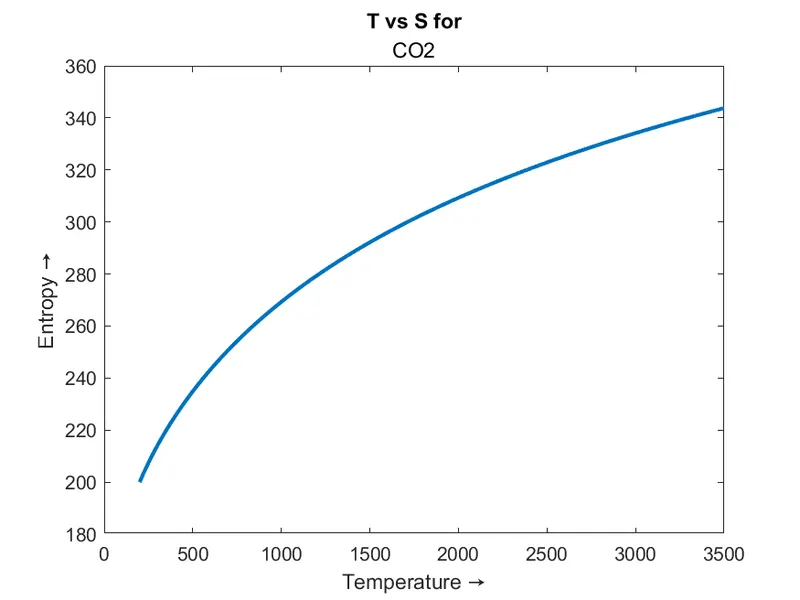
Plots of CO2
These are the plots obtained for T vs Cp, T vs H and T vs S for the species CO2.
The molecular weight of the species is calculated and is displayed in the command window.
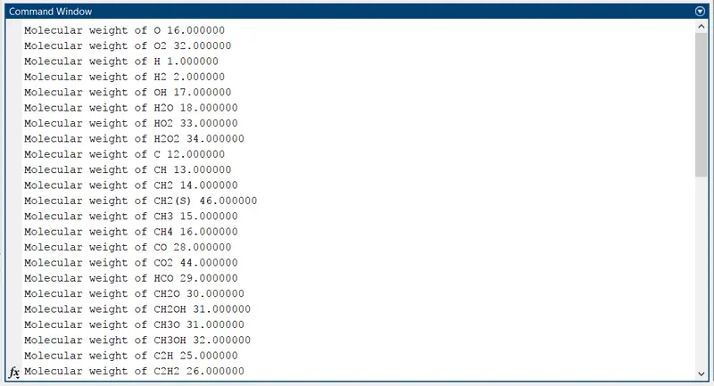
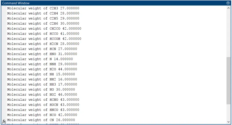
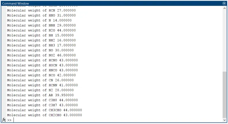
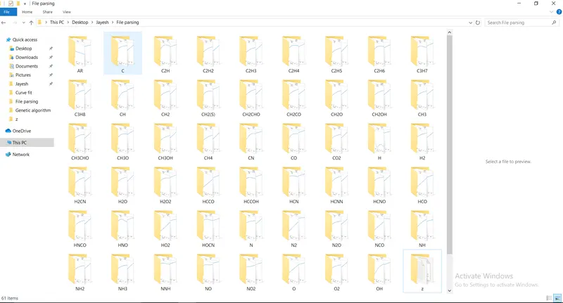
The sub- folders for each of the species was created in the current folder and the all the plots were saved into the sub-folders.
CONCLUSION:
Thus the required MATLAB program is written to complete the given task and the molecular weights of the species are displayed in the command window. With this, the process of writing data to a file and extract data from a given file is done using MATLAB.