Project - File Parsing NASA's Thermodynamic Data Using MATLAB
Project 1 – File Parsing
Aim - To write a MATLAB code to parse a NASA thermodynamic data file and calculate thermodynamic properties of various species .
Objective –
- MATLAB code for file parsing
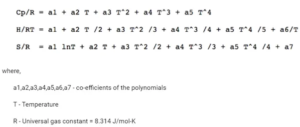
- Write a function that extracts the 14 coefficients and calculates the enthalpy, entropy and specific heats for all the species in the data file.
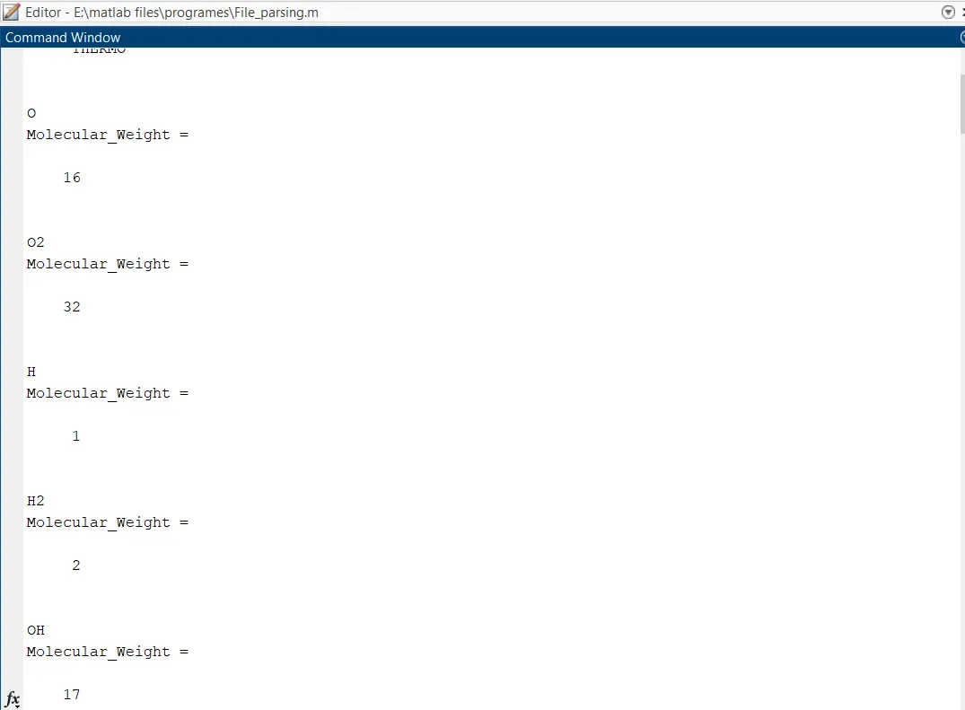
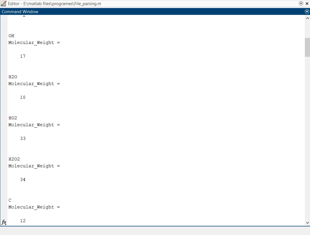
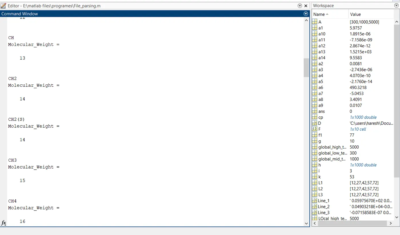
- Calculate the molecular weight of each species and display them
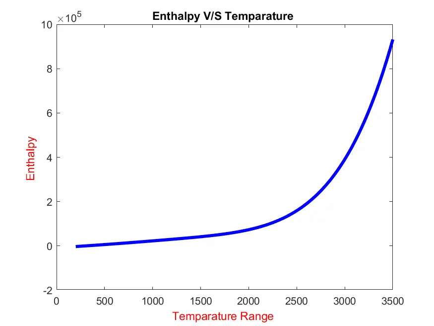
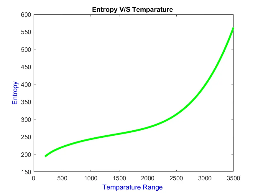
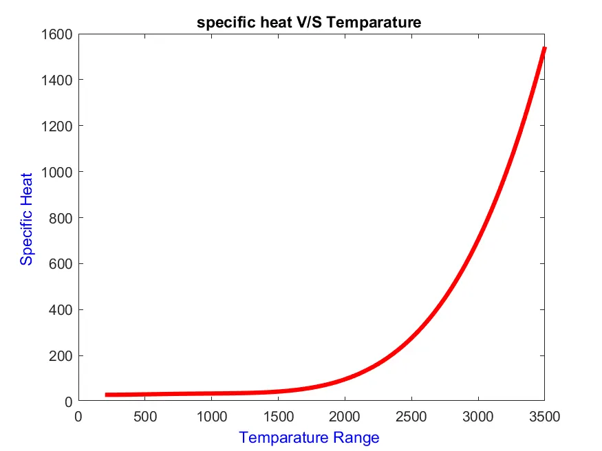
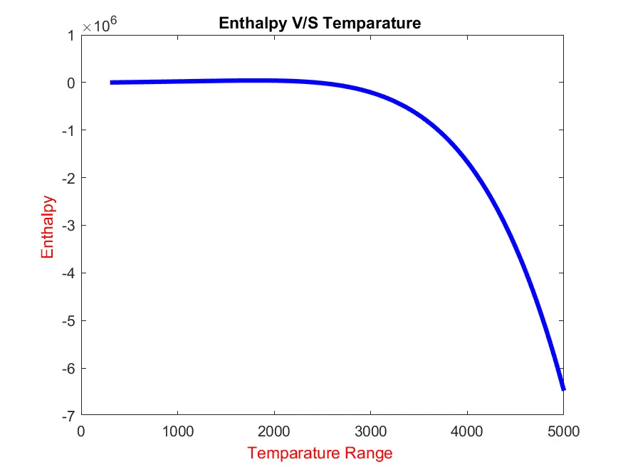
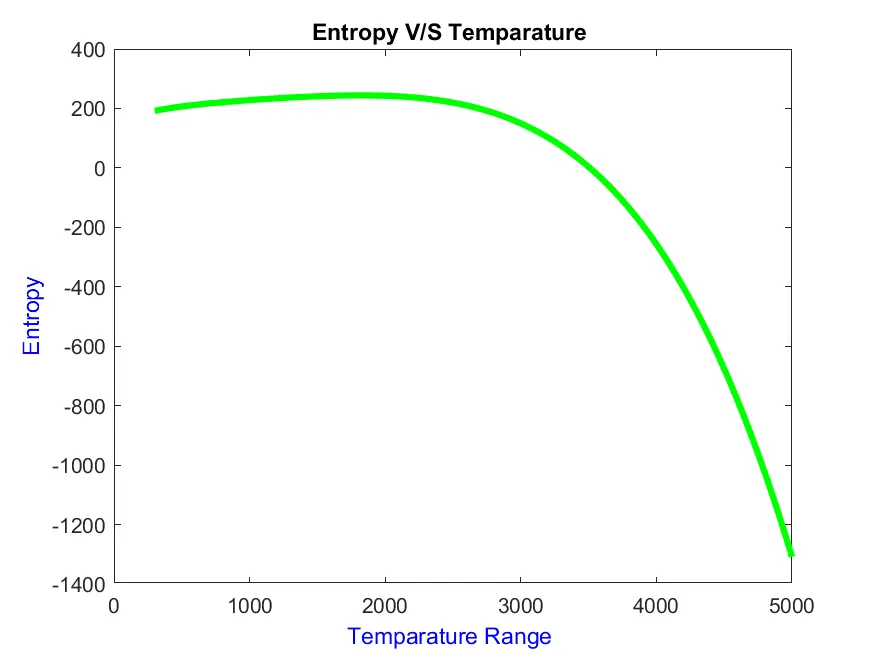
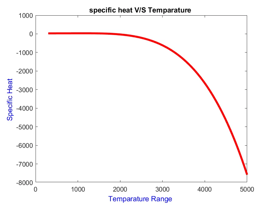
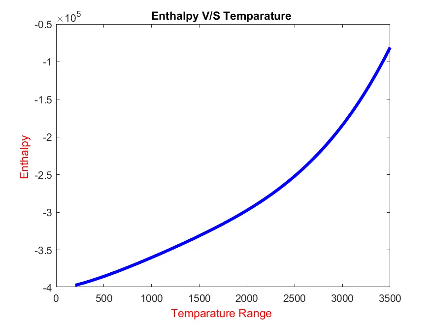
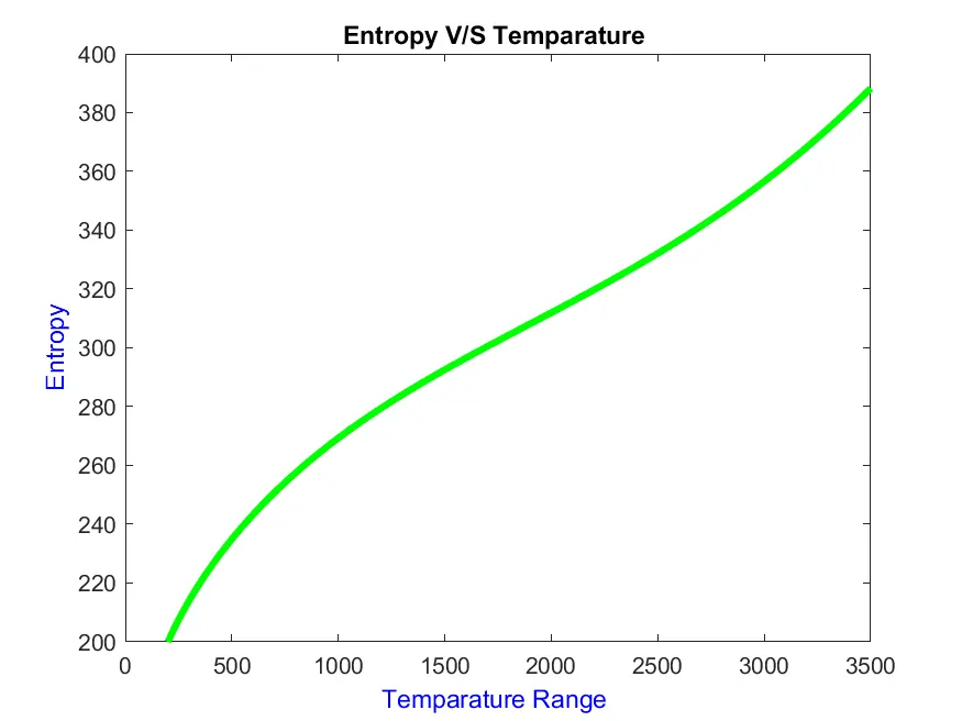
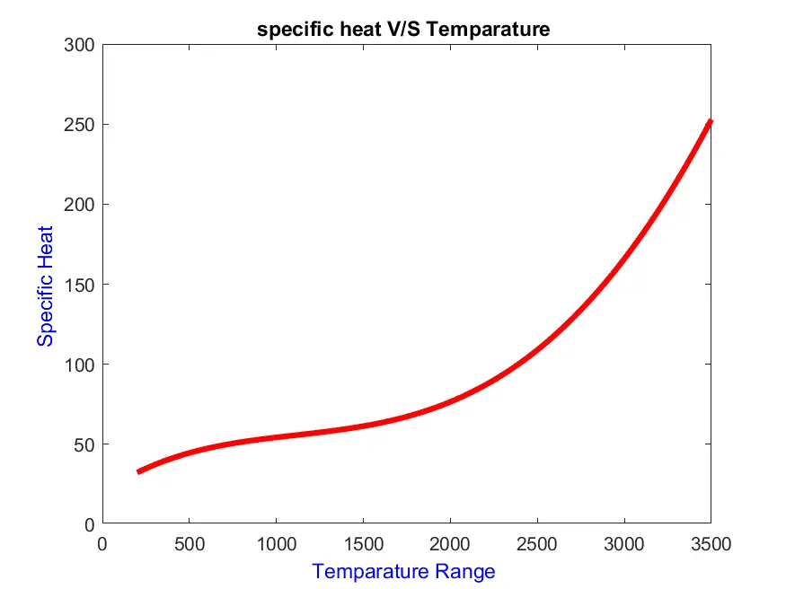
- Plot the Specific heat , Enthalpy and Entropy for the local temperature range (low temperature, high temperature) specific for each species..
Introduction -
File Parsing
In computer language parsing refers to analysis of the input code into its component parts in order to facilitate the writing of compilers and interpreters.
It basically means to read data from a text file and perform the analysis required.
Thermodynamic Properties -
Specific Heat –
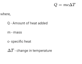
It is the amount heat per unit mass required to raise the temperature by one degree of Celsius
Entropy –
It is the measure of a system’s thermal energy per unit temperature that is unavailable for doing useful work . It is denoted by letter (S) .
Enthalpy -
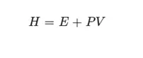
The sum of internal energy and the product of the pressure and volume of a thermodynamic system .
Governing Equations –
Main Code –
clc
clear all
close all

% opening the NASA Theermo file in read mode
f1  = fopen('File_Parsing_data.txt','r');

%skipping the first line
fgetl(f1)

%parsing the global temp
tline = fgetl(f1) ;
A = str2num(tline);

global_low_temp = A(1);
global_mid_temp = A(2);
global_high_temp = A(3);

% skipping the next three lines
for i = 1 : 3
    fgetl(f1) ;
end

% Parsing the co-efficients for calculation .
% Loop used from fist species to the  53rd species .


%%%   A for loop is to be used .........
for k = 1 : 53

  tline = fgetl(f1) ;
  F = strsplit(tline ,' ') ;
  species_name = F{1} ;
  g = length (F) ;
  % parsing the local temp ...
   LOcal_low_temp = str2double(F(g-3));
   LOcal_high_temp = str2double(F(g-2));
   LOcal_mid_temp = str2double(F(g-1));

   Line_1 = fgetl(f1) ;
   %identifing the chracter E ...
    L1 = strfind(Line_1,'E');
    % Reading the first line ....
    % Extracting co-efficients based on the position /.....
    a1 = str2num(Line_1(1:(L1(1)+3)));
    a2 = str2num(Line_1((L1(1)+4):(L1(2)+3)));
    a3 = str2num(Line_1((L1(2)+4):(L1(3)+3)));
    a4 = str2num(Line_1((L1(3)+4):(L1(4)+3)));
    a5 = str2num(Line_1((L1(4)+4):(L1(5)+3)));

    % Reading the second line ......
    Line_2 = fgetl(f1) ;
    L2 = strfind(Line_1,'E');
   % Reading the second  line ....
    a6 = str2num(Line_2(1:(L2(1)+3)));
    a7 = str2num(Line_2((L2(1)+4):(L2(2)+3)));
    a8 = str2num(Line_2((L2(2)+4):(L2(3)+3)));
    a9 = str2num(Line_2((L2(3)+4):(L2(4)+3)));
    a10 = str2num(Line_2((L2(4)+4):(L2(5)+3)));

    Line_3 = fgetl(f1) ;
    L3 = strfind(Line_1,'E');
   % Reading the second  line ....
    a11 =str2num (Line_3(1:(L3(1)+3)));
    a12= str2num (Line_3((L3(1)+4):(L3(2)+3)));
    a13= str2num (Line_3((L3(2)+4):(L3(3)+3)));
    a14= str2num (Line_3((L3(3)+4):(L3(4)+3)));

    % creating an array for temparature  of 1000 numbers //.......
     T = linspace(LOcal_low_temp , LOcal_high_temp ,1000) ;

     [cp ,h , s ] = coeff_file(a1,a2,a3,a4,a5,a6,a7,a8,a9,a10,a11,a12,a13,a14,T) ;

     %creating  a Directory and the folder to save the plots //.....
      old = pwd ;
     mkdir (['C:usershareshDocumentsMATLABProject-1species_name',species_name]) ;

     %pltting the data ...

     figure (1)

     grid on ;
     plot(T,cp ,'linewidth',3,'color','r');
     xlabel('Temparature Range ','color','b');
     ylabel('Specific Heat ','color','b');
     title('specific heat V/S Temparature ');


     figure (2)

     grid on ;
     plot(T,h ,'linewidth',3,'color','b');
     xlabel('Temparature Range ','color','r');
     ylabel('Enthalpy ','color','r');
     title('Enthalpy V/S Temparature ');


     figure (3)

     grid on ;
     plot(T, s ,'linewidth',3,'color','g');
     xlabel('Temparature Range ','color','b');
     ylabel('Entropy','color','b');
     title('Entropy V/S Temparature ');

     %saving the location to variable D ...
     D = (['C:usershareshDocumentsMATLABProject-1species_name',species_name]) ;
     cd(D)  %changing the directory ....

     % saving the plots. .....
     saveas(1,'Specific_Heat.png');
     saveas(2,'Enthalpy.png');
     saveas(3,'Entropy.png');
     cd('C:usershareshDocumentsMATLABProject-1species_name')

     % Printing the molecular weight of the species .....
     cd(old);
     fprintf('n')
     fprintf(species_name)
     Molecular_Weight = Moll_weight(species_name)

end
fclose(f1) ;
Function 1 -
% calculating the thermodynamic properties using the following function...
function[cp,h,s] =  coeff_file(a_1,a_2,a_3,a_4,a_5,a_6,a_7,a_8,a_9,a_10,a_11,a_12,a_1_3,a_14,T)
R = 8.314 ;
for i = 1:length(T)
    if T(i)<1000
        cp = (a_1 + (a_2.*T)+(a_3.*T.^2)+(a_4.*T.^3) + (a_5.*T.^4)).*R ;
        h =  (a_1 + (a_2.*T)./2+ (a_3.*(T).^2)./3+ (a_4.*(T).^3)./4+ (a_5.*(T).^4)./5+(a_6./T))*R.*T ;
        s =  (a_1.*log(T)+a_2.*T+(a_3.*T.^2)/2 + (a_4.*T.^3)./3+(a_5.*T.^4)./4+ a_7).*R;

    else
       cp = (a_8 + (a_9.*T)+(a_10.*T.^2)+(a_11.*T.^3) + (a_12.*T.^4)).*R ;
       h =  (a_8 + (a_9.*T)./2+ (a_10.*(T).^2)./3+ (a_11.*(T).^3)./4+ (a_12.*(T).^4)./5+(a_1_3./T))*R.*T ;
       s =  (a_8.*log(T)+a_9.*T+(a_10.*T.^2)/2 + (a_11.*T.^3)./3+(a_12.*T.^4)./4 + a_14).*R;

    end

end
Function 2 -
%To caculate the Molecular Weight ......
function [MW] = Moll_weight(species_name)

sp_name = upper(species_name);
a = { 'H' , 'C' , 'N' , 'O' , 'A' };
%defining the atomic wt of molecules ...
AW = [ 1  12  14   16  40  ] ;
MW = 0 ;
for i = 1 : length(sp_name)
     for j = 1 : length(a)
              if  strcmp(sp_name(i),a(j))
                  MW = MW + AW(j);
                  u = j;

               end
     end
n = str2double(sp_name(i) );    % This statement is used for  species_name having more than one molecule ...

if ( n > 1 )
    MW = MW +  AW(u) * (n-1)  ;

end


end


end
Explanation -
- The first three lines of the programe are used to refresh the workspace .
- Now opening the NASA data file in read mode using "r" , in "fopen" open . The position is now stored in variable "f1 " , which acts as an pointer for the file . This pointer is used to get the indivudual line in read mode .
- Using the "fgetl(f1)" command the first line is read .
- The second line contains the global temparatures which are stored into a variables .Using "str2num" which changes string to number .
- Then the rest three lines are skipped using for loop .
- Now to read the coe-fficients of different species , a "For loop" is used which is conditioned to run till "53" as there are a total of 53 species .
- Inside the loop the first line containg the species name and the local temparatures is read and stored.
- The next line is now read using "fgetl()" . The co-efficients are now stored into variables based on their positions using the "str2num" command .
- After storing the co-efficients , an array of Temparature is created containg the 1000 numbers From low_local_temparature to high_local_temparature range .
- The thermodynamic properties are now calculated using the "Function -1 " .
- Now the position of the current folder is stored to a variable using "pwd " command .
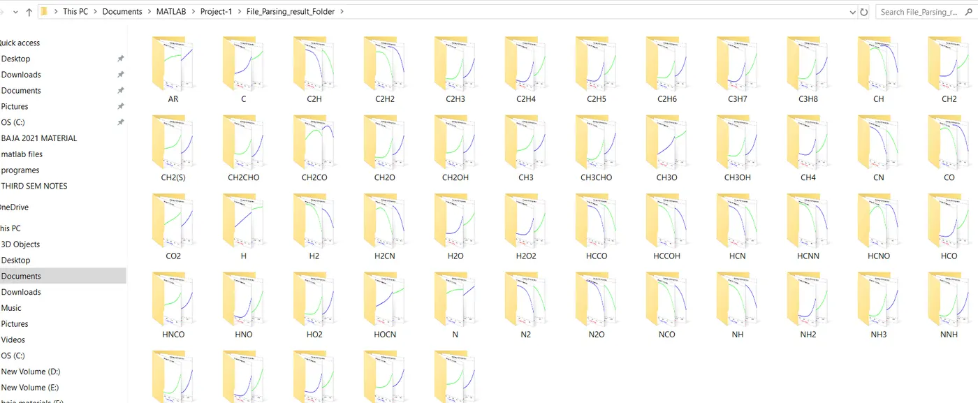
- A new directory is now created using the "mkdir" command also the folder with the species name is created .
- The result which was obtained is now used to plot the graph .
- The current directory is changed to the new one using "cd" command .
- The plots are then saved using "saveas" command by specifing the image name with the format .
- Now after saving the directory is again changed to the old one .
- This is done so that the molecular Weight of the species can be caculated using "Function -2 " .
- Thus the Molecular weight is now displayed on the command window .
Results -
Plots of O2 -
Plots of N2 -
Plots of CO2 -
Output -
Conclusion -
All the Objective of the code has been comleted Successfully .
References -
https://in.mathworks.com/help/matlab/ref/mkdir.html
https://in.mathworks.com/help/matlab/ref/cd.html
Thank You .