Project 1 - Parsing NASA thermodynamic data

AIM: To write a program in matlab to parse the NASA thermodynamic data file and then calculate the thermodynamic properties of
various gas species.

GOVERNING EQUATIONS:
The equations that we are going to use in the Functions to calculate cp, H,S are:

Where,
Cp=specific heat
R =molar gas constant
T=temperature
S=Entropy
H=Enthalpy
a=coefficients

OBJECTIVE:

• To write a function that extracts the 14 co-efficient and calculates the enthalpy ,entropy and specific heats for all species in the data file.
• Calculating the molecular weight of each species and displaying it in command window.
• Plotting cp, enthalpy and entropy for local temperature range specific for each species.
• Save the plot as images with appropriate names and dump them in separate folders for each species with suitable name.

INTRODUCTION:

Thermodynamics -

• Thermodynamics is a branch of physics that deals with heat,work and temprature, and their relation to energy,entropy, and the physical properties of matter and radiation. The behavior of these quantities is governed by the four laws of thermodynamics which convey a quantitative description using measurable macroscopic physical quantity, but may be explained in terms of microscopic constituents by statical mechanics.
• The initial application of thermodynamics to mechanical heat engine was quickly extended to the study of chemical compounds and chemical reactions. chemical thermodynamics studies the nature of the role of entropy in the process of chemical reaction and has provided the bulk of expansion and knowledge of the field.

LAWS OF THERMODYNAMICS-

1. Zeroth Law

   The zeroth law of thermodynamics states: If two systems are each in thermal equilibrium with a third, they are also in thermal equilibrium with each other.

2. First Law

   The first law of thermodynamics states: In a process without transfer of matter, the change in internal energy, , of a thermodynamic system is equal to the energy gained as heat, , less the thermodynamic work,, done by the system on its surroundings.

   
   .

3. Second Law

   A traditional version of the second law of thermodynamics states: Heat does not spontaneously flow from a colder body to a hotter.

4. Third Law

   The third law of thermodynamics states: As the temperature of a system approaches absolute zero, all processes cease and the entropy of the system approaches a minimum value.

Absolute zero, at which all activity would stop if it were possible to achieve, is −273.15 °C (degrees Celsius), or −459.67 °F (degrees Fahrenheit), or 0 K (kelvin), or 0° R (degrees Rankine ).

PARSING DATA:
Parsing means to make something understandable. For programming this means to convert information represented in one
form into another form that's easier to work with. This is done by partially analysing the data, understanding its underlying
structure (by making some assumptions based on what you're expecting to see), and then explicitly representing that structure
in the code.
Parsing a file means reading in a data stream of some sort and building an in memory model of the semantic content of that
data. This aims at facilitating perfoming some kind of transformation on the data.

MATLAB CODE

% NASA Thermodynamic data 

%clear all the previous data or stores values
clear all
close all
clc

%R=molecular gas constant
R=8.314;

%Open the the THERMO.dat file
f1=fopen('THERMO.dat','r')

%skip the first line
%skip next three lines use for loop
for i=1:5    
l=fgetl(f1)
end

for i = 1:53
l_1 = fgetl(f1)
a = strsplit(l_1,' ')
species = (a{1})

b = strfind(l_1,'.');          %find the position of dots
low_temp = l_1(b(1)-3:b(1)+3);  %find the low teprature value using positin of dot
low_temp = str2num(low_temp)   %convert the string into number

high_temp= l_1(b(2)-4:b(2)+3);
high_temp = str2num(high_temp)

mid_temp= l_1(b(3)-4:b(3)+3);
mid_temp = str2num(mid_temp)

datal_1=fgetl(f1)
datal_2=fgetl(f1)
datal_3=fgetl(f1)

b = strfind(datal_1,'E'); 
c= strfind(datal_2,'E'); 
d = strfind(datal_3,'E'); 

t1=datal_1(1:b(1)+3);
t2=datal_1(b(1)+4:b(2)+3);
t3=datal_1(b(2)+4:b(3)+3);
t4=datal_1(b(3)+4:b(4)+3);
t5=datal_1(b(4)+4:b(5)+3);

t1=str2num(t1);
t2=str2num(t2);
t3=str2num(t3);
t4=str2num(t4);
t5=str2num(t5);

t6=datal_2(c(1)-10:b(1)+3);
t7=datal_2(c(1)+4:b(2)+3);
t8=datal_2(c(2)+4:b(3)+3);
t9=datal_2(c(3)+4:b(4)+3);
t10=datal_2(c(4)+4:b(5)+3);

t6=str2num(t6);
t7=str2num(t7);
t8=str2num(t8);
t9=str2num(t9);
t10=str2num(t10);

t11=datal_3(d(1)-11:b(1)+3);
t12=datal_3(d(1)+4:b(2)+3);
t13=datal_3(d(2)+4:b(3)+3);
t14=datal_3(d(3)+4:b(4)+3);

t11=str2num(t11);
t12=str2num(t12);
t13=str2num(t13);
t14=str2num(t14);

T=linspace(low_temp,high_temp,100);

%initializing specific heat,entropy and enthalpy values for high and low
%temprature range
for i=1:length(T)
    if T(i)>mid_temp
        cp(i)=R*(t1+t2.*T(i)+t3.*T(i)^2+t4.*T(i)^3+t5.*T(i)^4);
        H(i)=R*T(i).*(t1+((t2*T(i))/2)+((t3*T(i).^2)/3)+((t4*T(i).^3)/4)+((t5*T(i).^4)/5)+t6/T(i));
        S(i)=R*(t1*log(T(i))+t2*T(i)+((t3*T(i).^2)/2)+((t4*T(i).^2)/3)+((t5*T(i).^3)/3)+((t6*T(i).^4)/4)+t7);
    else 
        cp(i)=R*(t8+t9.*T(i)+t10.*T(i)^2+t11.*T(i)^3+t12.*T(i)^4);
        H(i)=R*T(i).*(t8+((t9*T(i))/2)+((t10*T(i).^2)/3)+((t11*T(i).^3)/4)+((t12*T(i).^4)/5)+t13/T(i));
        S(i)=R*(t8*log(T(i))+t9*T(i)+((t10*T(i).^2)/2)+((t11*T(i).^2)/3)+((t12*T(i).^3)/3)+((t13*T(i).^4)/4)+t14);
    end

end

%molecular weight of spices

[w]=mol_weight(species)
fprintf('Molecular weight of %s = %f', species, w);

% Saving in a folder
cd('D:\skill lync\matlab\project 1 -thermodynamics\graphs')
mkdir(species)
cd(species)

%plotting specific heat vs temprature
figure(1)
plot(T,cp,'linewidth',3);
title(sprintf('Variation of specific Heat with Temprature for %s',species))
ylabel('specific heat(cp)')
xlabel('Temprature(T)')
saveas(figure(1),'cp vs T.png') 

%plotting enthalpy vs temprature
figure(2)
plot(T,H,'linewidth',3)
title(sprintf('Variation of Enthalpy with Temprature for %s',species))
 ylabel('ENTHALPY (H)')
 xlabel('Temprature(T)')
 saveas(figure(1),'H vs T.png') 
 
%plotting entrophy vs temprature
 figure(3)
 plot(T,S,'linewidth',3)
title(sprintf('Variation of Entrophy with Temprature for %s',species))
ylabel('ENTROPHY (S)')
xlabel('Temprature(T)')
saveas(figure(1),'S vs T.png') 

cd('C:\Users\AMANDEEP ROHILLA\Documents\MATLAB')

end

function to find molecular weight

%function for finding the molecular weight 

function [w]=mol_weight(species)
atomic_names=['H', 'C', 'O', 'N', 'A']; 
atomic_weights=[1.00784,12.0107,15.999,14.0067,39.948];
w=0;

for i=1:length(species)

for j=1:length(atomic_names)

if strcmpi(species(i), atomic_names (j))
    w=w+atomic_weights(j);

pos=j;

end
end
n=str2double(species(i));
if n>1
    
    w =w+atomic_weights(pos)*(n-1);

end
end
%fprintf('Molecular weight of %s = %f', species, w);

end

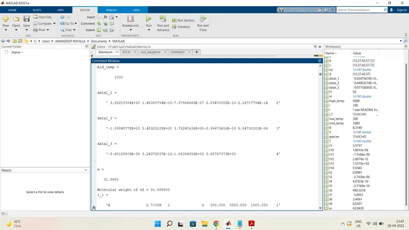
Molecular weight for 02

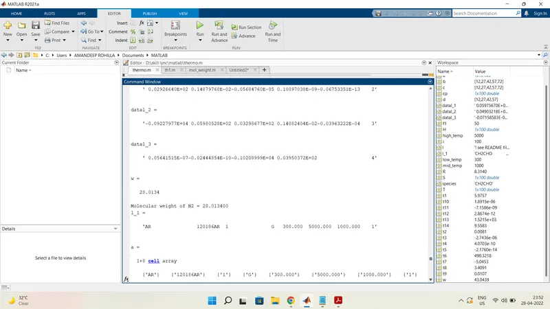
Molecular weight for N2

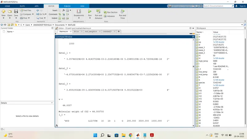
Molecular weight for C02

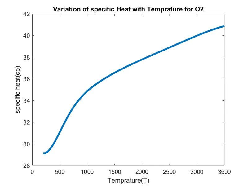
GRAPH

1. O2

CP VS T

H VS T

S VS T

2. N2

CP VS T

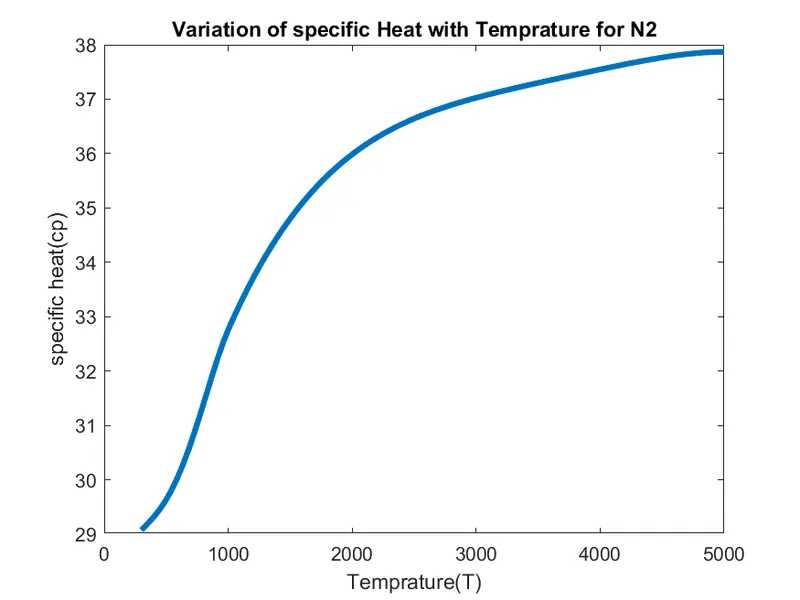
H VS T

S VS T

3. C02

CP VS T

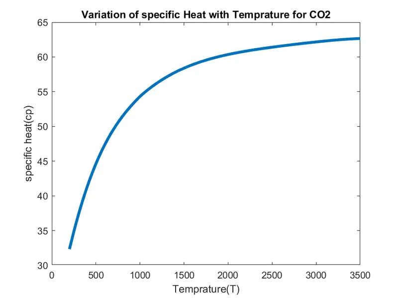
H VS T

S VS T

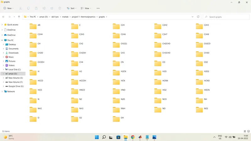
FOLDER CREATION

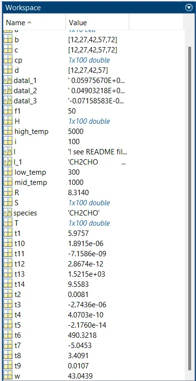
Workspace window

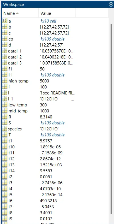
CODE EXPLANATION

• Initially the value of ‘R’ is being defined.
• Then we use a command to open the file ‘THERMO.dat’ .
• Further we use the ‘fgetl’ to start reading the lines and after reading the first two lines, from the second line converting thestrings to numbers and assigning global (low,mid and high) temperatures.
• Then we have written a command to get the temperature range for calculation and plotting purpose.
• Then again using the fgetl command to go to thel next 3 lines and skipping it.
• Then we use a for loop to get 53 species and their temperatures (low, mid, high) and the 14 coefficients.
• In the for loop we again use the fgetl command and then the next line is read and from that line the species name, the three local temperatures are read and stored.
• Then we use fgetl command to go to further line and get the first 7 coefficients and store them. Similarly using the fgetl
  command we move to the next two lines and get the remaining coefficients.
• Then after getting the 14 coefficients, we use these coefficients and by calling the functions we calculate cp,H,S.
  Further we use the Molecular weight function and calculate molecular weight for that species.
• Further I have used a command to change the directory so that I can save the files at a particular location.After changing the directory I have used ‘mkdir' to create a new folder with the name of the current species and then a ‘cd’ command to make mkdir as the current directory.
• Then further we use plot command to plot temperature vs (cp,enthalpy,entropy) .
• In this plotting we use the figure command to get the three different plots and saveas command to save the figures in the Then again we change our directory to again start the loop. So the loop continues to function till we get all the 53 species and then gets terminated.

Result:- succesfully create Matlab programme to calculates the enthalpy, entropy and specific heats for all the species in the data file and molecular weight of the spices.

CONCLUSION: So here we were able to parse the data from the THERMO.dat file. Then using this data we were able to calculate the thermodynamic
properties and also make plots for these properties with respect to the temperature.

REFERENCES:
https://www.mathworks.com/matlabcentral/answers/341599-create-folder-and-keep-files