Project 1 - Parsing NASA thermodynamic data

Aim-Write a code in Matlab to parse the NASA thermodynamic data file and then calculate the thermodynamic properties of various gas species

File Parsing :

Parsing, syntax analysis, or syntactic analysis is the process of analyzing a string of symbols, either in natural language, computer languages or data structures, conforming to the rules of formal grammar. The term parsing comes from Latin pars meaning part of speech. Within computational linguistics the term is used to refer to the formal analysis by a computer of a sentence or other string of words into its constituents, resulting in a parse tree showing their syntactic relation to each other, which may also contain semantic and other information. Some parsing algorithms may generate a parse forest or list of parse trees for a syntactically ambiguous input. Parsing a file means reading in a data stream of some sort and building an in-memory model of the semantic content of that data. This aims at facilitating performing some kind of transformation on the data.

NASA thermodynamics file :

NASA thermodynamics file  NASA_THERMODYNAMIC_FILE where the temperature range and 53 species are given in this data and each species contains 14 coefficients and temperature ranges and we have to parse these 14 coefficients to find Specific heat.

Entropy and Enthalpy using formula as-

where-

• R=universal gas constant
• T=Temperature
• Cp=Specific heat (KJ)
• S=Entropy(KJ/mol-K)
• H = Enthalpy(KJ/mol)
• a(I)= coefficients where,i=1:14

Function code  for specific heat :

%function code to find the specific heat

function cp=specific_heat(a1,a2,a3,a4,a5,a8,a9,a10,a11,a12,T,R,mid_globel_temp)

T>mid_globel_temp;

cp = R*(a1+(a2*T)+(a3*(T).^2)+(a4*(T).^3)+(a5*(T).^4));

cp = R*(a8+(a9*T)+(a10*(T).^2)+(a11*(T).^3)+(a12*(T).^4));

end​

specific heat-

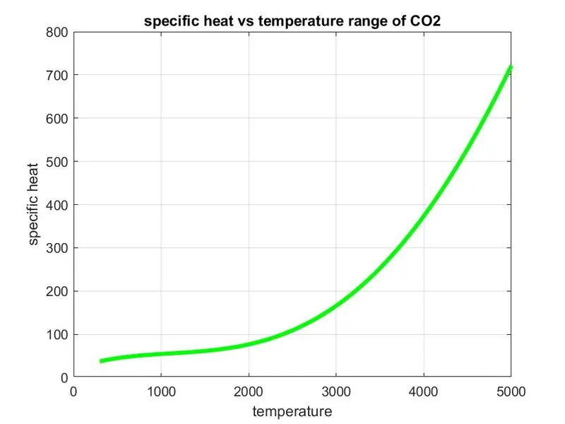
The specific heat is the amount of heat per unit mass required to raise the temperature by one degree Celsius. The relationship between heat and temperature change is usually expressed in the form shown below where c is the specific heat.

Cp = R*(a1 + (a2*T) + (a3*(T).^2) + (a4*(T).^3) + (a5*(T).^4))

code explanation :

• at first, we have to use the  word Function to start the function command
• Now we will find the Specific heat by creating a Specific heat function and assigning its related formula coefficient from 14 coefficients, Gas constant, Temperature and mid-temperature.
• and then we want to create a templet and this is a code templet and name for the templet
• we are going to name the code templet specific_heat
• we are going to use this formula to solve the equation.
• so whenever we want to substitute different values we just call this function and then pass in the right values
• then we have to save the function while saving the name of the function and the name of the file should exactly be the same
• the calling the function means using the function and using the templates with the appropriate values
• we have to ensure the no of inputs we provide match the orders of inputs also match
• end word is used to end the function command.

Function code for Entropy :

%function code to find the entropy

function s = entropy (a1,a2,a3,a4,a5,a7,a8,a9,a10,a11,a12,a14,T,R,mid_global_temp)
(T < = mid_global_temp)

s = R*(a1.log(T)+(a2*T)+((a3(T).^2)/2)+((a4*(T).^3)/3)+((a5*(T).^4)/4)+a7);

s = R*(a8.log(T)+(a9*T)+((a10(T).^2)/2)+((a11*(T).^3)/3)+((a12*(T).^4)/4)+a14);
end

Entropy :

the measure of a system's thermal energy per unit temperature that is unavailable for doing useful work. Because work is obtained from ordered molecular motion the amount of entropy is also a measure of the molecular disorder, or randomness, of a system.

S = R*(a1.log(T) + (a2*T) + ((a3(T).^2)/2) + ((a4*(T).^3)/3) + ((a5*(T).^4)/4) + a7)

ENTHALPY :

%function code to find the Enthalpy

function H= enthalpy(a1,a2,a3,a4,a5,a6,a8,a9,a10,a11,a12,a13,T,R,mid_globel_temp)

(T<=mid_globel_temp);

H = R*T.*(a1+((a2.*T)/2)+((a3*(T).^2)/3)+((a4*(T).^3)/4)+((a5*(T).^4)/5)+((a6./T)))

H = R*T.*(a8+((a9*T)/2)+((a10*(T).^2)/3)+((a11*(T).^3)/4)+((a12*(T).^4)/5)+((a13./T)))

end

ENTHALPY :

Enthalpy , a property of a thermodynamic system, is equal to the system's internal energy plus the product of its pressure and volume. In a system contained so as to prevent mass transfer, for processes at constant pressure, the heat absorbed or released equals the change in enthalpy.

H = R*T.(a1 + ((a2*T)/2) + ((a3(T).^2)/3) + ((a4*(T).^3)/4) + ((a5*(T).^4)/5) + ((a6./T)))

MAIN CODE :

%parsing NASA tharmodynamic data
close all
clear all
clc

%input
R = 8.314;

%opening the filing and reading the file data

f1 = fopen('THERMO.dat','r');
header_line = fgetl(f1);

%getting the globel temprture of the file

globel_temp = fgetl(f1);

%splitting the line

split_temp = strsplit(globel_temp);

%converting the string sells to the number

low_globel_temp = str2double(split_temp{2});
mid_globel_temp = str2double(split_temp{3});
high_globel_temp = str2double(split_temp{4});

%getting varisous temprature range between low and high temperature

temp = linspace(low_globel_temp,high_globel_temp,1000);
T = temp;

%skipping the header comment 

fgetl(f1);
fgetl(f1);
fgetl(f1);

%reading the 53 species

for j=1:53
    tline = fgetl(f1);
    
%splitting
A=strsplit(tline,' ');

%to read the name of the species
species=(A{1});

%converting the strings to the number

low_temp=str2double(A{6});
mid_temp=str2double(A{8});
high_temp=str2double(A{7});

tline1=fgetl(f1);

%finding the E string in the line

a=strfind(tline1,'E');

% finding high temperature coefficients

a1 = tline1(1:a(1)+3);
a1 =  str2double(a1);

a2 = tline1(a(1)+4:a(2)+3);
a2 =  str2double(a2);

a3 = tline1(a(2)+4:a(3)+3);
a3 =  str2double(a3);

a4 = tline1(a(3)+4:a(4)+3);
a4 =  str2double(a4);

a5 = tline1(a(4)+4:a(5)+3);
a5 =  str2double(a5);

tline2 = fgetl(f1);
b = strfind(tline2,'E');

a6 = tline2(1:b(1)+3);
a6 = str2double(a6);

a7 = tline2(b(1)+4:b(2)+3);
a7 = str2double(a7);

%find lower temperature coefficients

a8 = tline2(b(2)+4:b(3)+3);
a8 = str2double(a8);

a9 = tline2(b(3)+4:b(4)+3);
a9 = str2double(a9);

a10 = tline2(b(4)+4:b(5)+3);
a10= str2double(a10);

tline3 = fgetl(f1);

c = strfind(tline3,'E');

a11 = tline3(1:c(1)+3);
a11 = str2double(a11);

a12 = tline3(c(1)+4:b(2)+3);
a12 = str2double(a12);

a13 = tline3(c(2)+4:b(3)+3);
a13 = str2double(a13);

a14 = tline3(c(3)+4:b(4)+3);
a14 = str2double(a14);

%calculating specific heat
cp=specific_heat(a1,a2,a3,a4,a5,a8,a9,a10,a11,a12,T,R,mid_globel_temp);

%calcullating Entropy
s=entropy(a1,a2,a3,a4,a5,a7,a8,a9,a10,a11,a12,a14,T,R,mid_globel_temp);

%calcullating Enthalpy
H=enthalpy(a1,a2,a3,a4,a5,a6,a8,a9,a10,a11,a12,a13,T,R,mid_globel_temp);

%calculating the molecular weight of the species
W = molecular_weight(species);

%writing of molecular weight file
molecular_weight_file = fopen('Molecular weight.txt','w');
fprintf(molecular_weight_file,'Moleculer weight of %s is %d',species,W);

%closing of the file
fclose(molecular_weight_file);

%plotting cp,H,s with temperature

%saving folder
cd('C:\Users\91733\OneDrive\Documents\MATLAB\mat');

%creating directory
mkdir(species);
cd(species);

%ploting 1cp vs T

figure(1)
plot(T,cp,'LineWidth',3,'Color','g');
xlabel('temperature');
ylabel('specific heat');
title(sprintf('specific heat vs temperature range of %s',species));
grid on;
saveas(figure(1),'specific heat.jpg');

% Plot 2 S vs T

    figure(2)
    plot(T,s,'linewidth',2,'color','b');
    xlabel('Temperature');
    ylabel('Entropy');
    title(sprintf('Entropy vs Temperature range of %s',species));
    grid on
    saveas(figure(2),'Entropy.jpg');


    % Plot 3 Cp vs T

    figure(3)
    plot(T,H,'linewidth',2,'color','r');
    xlabel('Temperature');
    ylabel('Enthalpy');
    title(sprintf('Enthalpy vs Temperature range of %s',species));
    grid on
    saveas(figure(3),'Enthalpy.jpg');

    %Changing directory to Original matlab path

    cd('C:\Users\91733\OneDrive\Documents\MATLAB\mat') ;
    % Molecular weight

    W = molecular_weight(species);
end

CODE EXPLAINATION :

-Firstly, we will Input the parameter R and we will open a file THERMO.dat file and reading this file using fopen       command.
-Then, we will read first THERMO using fgetl command and then we read temperature file and we will split the       temperatures using strsplit command to convert it into cell array and then we will convert this string to number   using str2num command to find low, high and mid temperatures.
-Then we will assign temperature range using linspace command. Then we run loop to skip command lines the       data file using fgetl command inside the loop.
-Now, we will run the loop to find 53 element in the data file by assigning fgetl command and then spliting into     the cell array to find the species line and then find the species name and then find the number of the                 temperatures in the species line.
-Then we read the new line. In order to read the coefficient in the data file we will first find the 'E' string using       strfind command to find before and after numbers of the coefficients then we will find remaining 14 coefficients     and convert them to numbers from strings.
-Out of which we will find the first 7 Coefficients which are for Higher temperature and then Second 7   Coefficients which are for Lower temperature.
-Now we will specify Specific heat Cp, Entropy S, Enthalpy H functions to find these parameters using these 14     coefficients for Lower and higher Temperature. then we will specify molecular weight W function to find the   molecular weight of the different species.
-Now we will write the Molecular weight.txt file and fprintf all the molecular weights of the species. and then   close the txt file using fclose command.
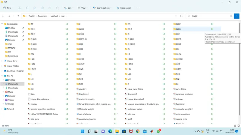
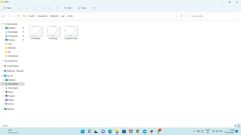
-Now we change the directory using cd command and then creating directory folder where we have to save our   files using mkdir command and then we will change the directory to this created folder.
-Now, we will plot Specific heat, Entropy and Enthalpy with the Temperature for different species. We we will use   scanf command to in the title command to create different species title.
-Then we will use saveas command to save the plots of different species in the directory folder. Now we will   change the directory to which our main code file runs in the MATLAB.

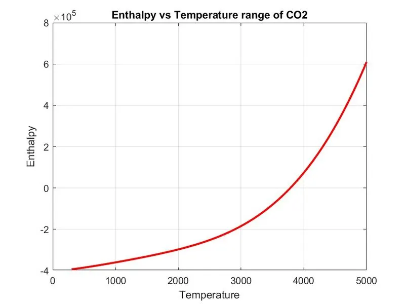
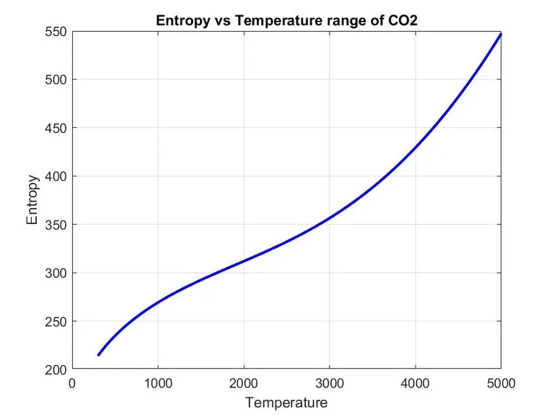
PLOTS OF CO2 :

PLOTS OF N2 :

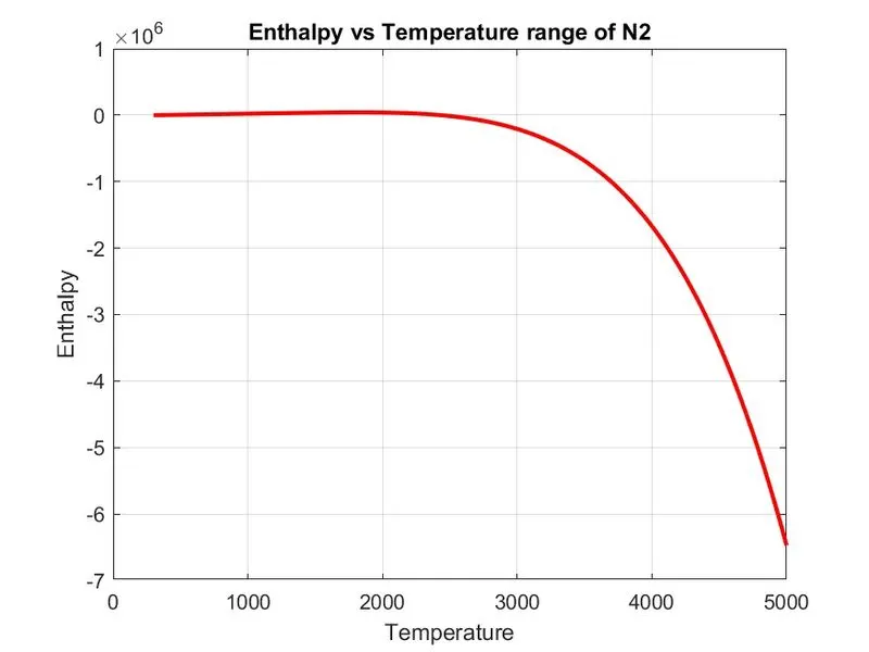
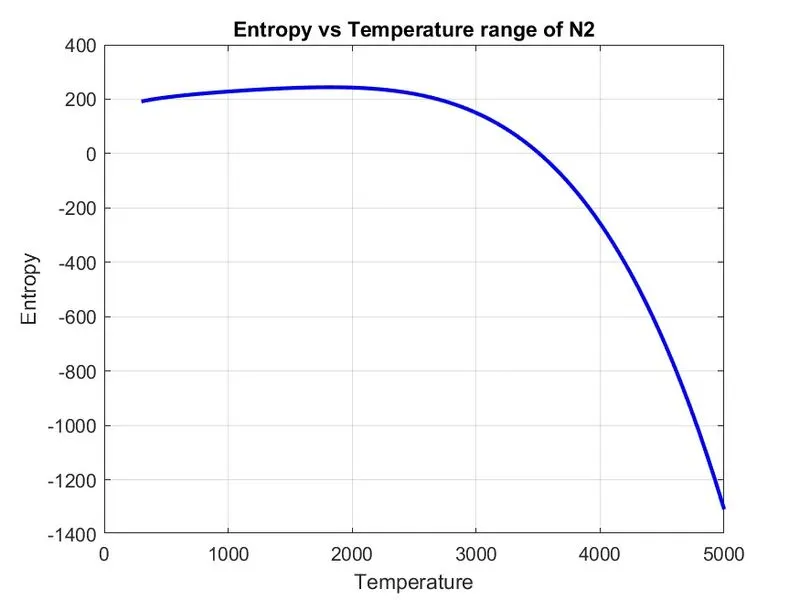
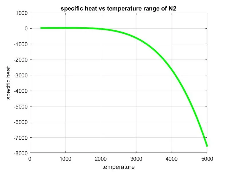
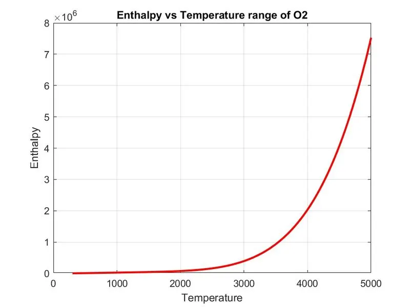
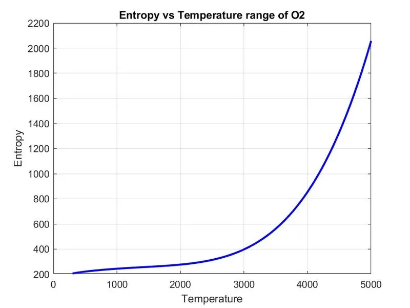
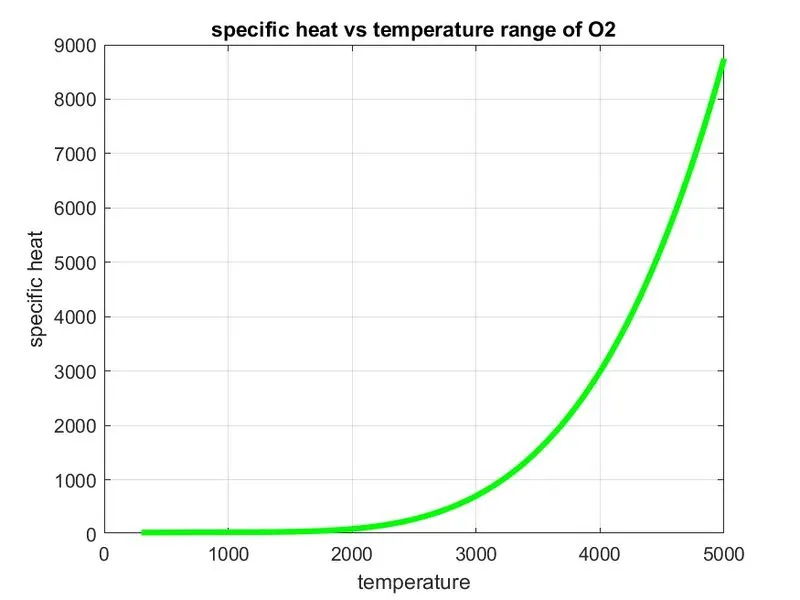
PLOTS OF O2 :

FOLDERS SAVED :