Project-1: Modelling an electric Car with Li-ion battery

Final Project - Modelling an Electric Vehicle with a Lithium-Ion Battery

Aim:

To create a SIMULINK model of an electric vehicle (EV) that is powered by a lithium-ion battery with speed control implementation using a PID controller.

Theory:

Electric Vehicles (EVs) are vehicles that are powered by electrical energy. The main components of an EV are a motor/generator, motor controller, power converters, wheels, and batteries. The electric motor is used to provide the power required for the wheels to move and provide traction. The motor controller and power converters work together to control the amount of power that is delivered to the motor. The batteries store the electrical energy needed to power the motor.

Traditional vehicles use an Internal Combustion (IC) engine which is powered by chemical energy from fossil fuels such as petrol or diesel. Traditional vehicles still represent the majority of all the vehicles being used around the world, however, there are various disadvantages in their use. For instance, the gaseous emissions such as carbon dioxide from those vehicles pose various environmental threats such as air pollution. These threats are said to be related to global warming. In addition, traditional vehicles will only be in demand till the availability of fossil fuels is exhausted. Fossil fuels are an exhaustible fuel source with negative environmental effects in its production as well as its utilization. The biggest advantage in using fossil fuels is their excellent energy density. Fossil fuels are capable of storing enormous amounts of energy per unit weight or unit volume which makes them ideal for efficiency. EVs utilize electrical energy stored in batteries as their power source and till date, even battery technologies are yet to reach the same energy density as fossil fuels were capable of.

In this project, I will model an EV in SIMULINK using the powertrain blockset and simscape blocks. This model will implement speed control using a PID controller block. The input to this model will be a Wide Open Throttle (WOT) drive cycle. The output of this model will be blocks that show the total distance travelled by the model and the speed of the vehicle during a 30 second simulation period. The speed data will reflect both the actual speed of the vehicle and the command speed from the drive cycle data.

System Level Configuration:

To model the EV in SIMULINK, we need to model the individual components of an EV such as the motor, controller, power converters, wheels, and batteries. All of these components are available as blocks from the simscape and powertrain blocksets. The various components of the EV will be modelled and explained in the sections below:

Vehicle Body

To model the body of the EV, we need to insert the vehicle body block shown in the image below:

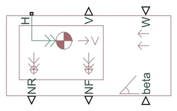
This block has 6 ports which represent various aspects of the modelling of the vehicle body:

• H - This stands for hub and allows us to connect the hubs of the wheels of the vehicle to the body.
• V - This stands for velocity and outputs the velocity of the vehicle.
• W - This represents wind velocity and allows us to model a headwind (against the front of the vehicle) acting on the velocity by giving a speed for it.
• NR - This represents the normal force on the rear wheels of the vehicle.
• NF - This represents the normal force on the front wheels of the vehicle.
• beta - This represents the grade (incline) of the surface that the vehicle travels on, as an angle to the horizontal.

Double-clicking the vehicle body block opens the block parameters shown below:

Main Tab

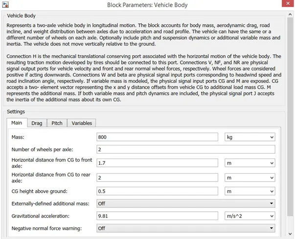
From the "Main" tab, here, we can model the basic parameters of the vehicle such as mass, number of wheels per axle and even gravitational acceleration. For my model, I am using a mass of 800kg, 2 wheels per axle (total of 4 wheels), and a gravitational acceleration of 9.81 metres per second squared.

Drag Tab

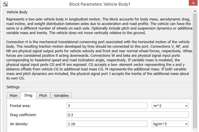
From the "Drag" tab, we can model the frontal area, drag coefficient, and the air density. I have used a frontal area, drag coefficient, and air density of 3, 0.3, and 1.18 respectively.

Wind Velocity & Slope

From the "W" and "beta" ports on the vehicle body block, I have used a "PS-Constant" block to model the effect of the wind velocity and the slope.

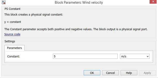
For the wind velocity, I have used a constant value of 5.

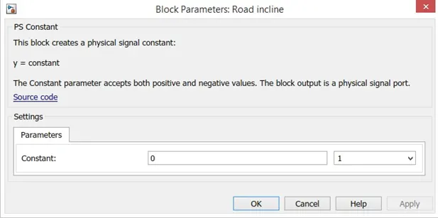
For the road incline, I have used a constant value of 0.

Velocity Subsystem

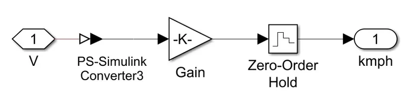
From the "V" port on the vehicle body bock, I have created a subsystem. This is because by default, this port will output the vehicle speed in miles per hour. For personal preference, I have created the subsystem to get the output speed in kilometres per hour. This system consists of a PS-Simulink converter block, a gain block, and a zero-order hold block. The gain block uses a factor of 1.6 to convert the speed from miles per hour to kilometres per hour. The PS-Simulink converter block is used to convert the physical signal of speed to a SIMULINK signal to be displayed on the scope block.

This subsystem is shown below:

Tires

In this model, I have used the "Magic Formula" tires. There are various tire blocks that can be used, but the advantage of the magic formula ones is that they enable us to model the longitudinal behavior of tires on a highway. This block is shown below:

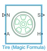
This block has 4 ports which represent various factors that can be modelled:

• N - This port represents the normal force on the tire and the downward direction is considered positive.
• S- This port represents the slip acting on the tire.
• A - This port represents the axle and is the mechanical rotational conserving port for the wheel axle.
• H - This port represents the hub and is the mechanical translational conserving port for the wheel hub.

Double-clicking the magic formula tire block, opens the block parameters window shown below:

Main

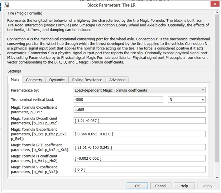
In the "Main" tab, we can model parameters such as tire nominal vertical load, and various coefficients. All values are kept as default.

Geometry

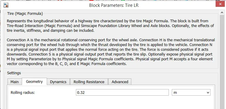
In the "Geometry" tab, we can model the rolling radius of the tire.

Dynamics

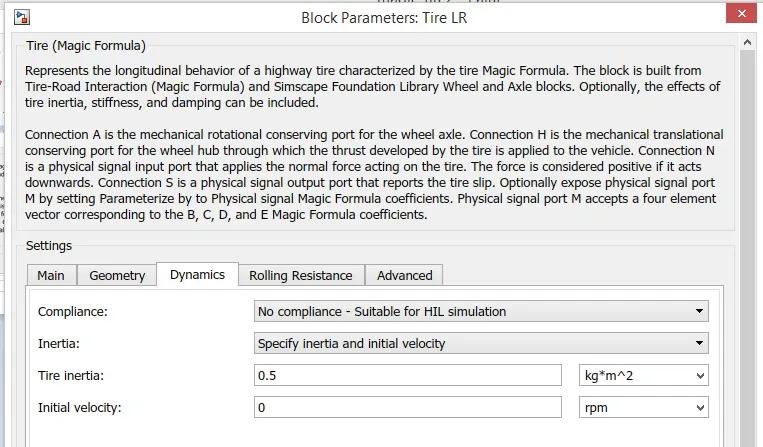
In the "Dynamics" tab, we can model parameters such as the tire inertia and initial velocity.

Rolling Resistance

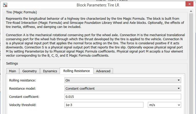
In the "Rolling Resistance" tab, we can model the effect of rolling resistance more closely. In this model, I have turned on the effect of rolling resistance, and have used a constant rolling resistance coefficient.

Gear

In this section, I have modelled the transmission of the EV. To simplify the transmission system of the EV model, I have used a "Simple Gear" block which uses a fixed gear ratio with no inertial effects. This block is shown below:

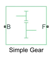
Double-clicking this block, opens the block parameters where we can model additional parameters of the gear.

Main

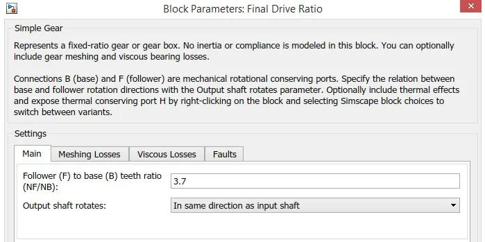
In the "Main" tab, we can model the follower to base teeth ratio and the direction of rotation of the output shaft. These settings were kept as default.

Meshing Losses

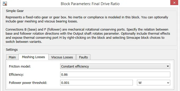
In the "Meshing Losses" tab, we can model the frictional effects on the gear. I have used a constant efficiency friction model with an efficiency of 0.86 and a follower power threshold of 0.001.

Side Shaft

The side shaft block is used to create inertial effects on the simple gear. This block only has one mechanical rotational conserving port and the positive direction of the block is from the port to the reference point (simple gear block). The side shaft block is shown below:

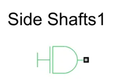
Double-clicking the side shaft block, opens the side shaft block parameters shown below:

Parameters

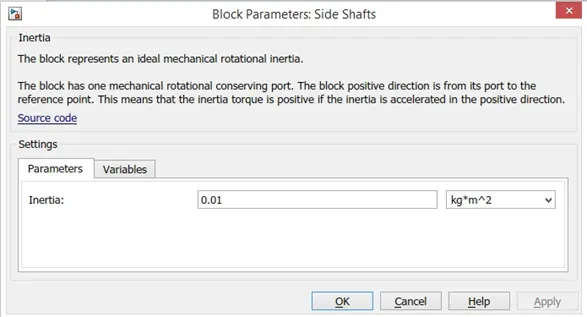
In the "Parameters" tab, we can model the inertia of the side shaft. The default value of 0.01 is used.

Vehicle Body Subsystem

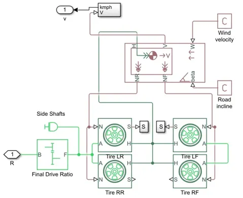
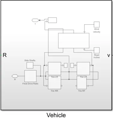
The full vehicle body system is shown in the image above with all the aforementioned blocks connected together. Four magic tire block are used to represent a four-wheeled vehicle. This system is then converted to a subsystem shown in the image below:

Motor

For my EV model, I am using a DC motor block which is shown below:

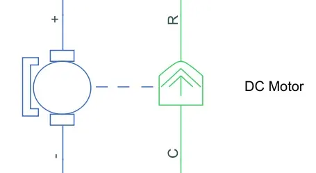
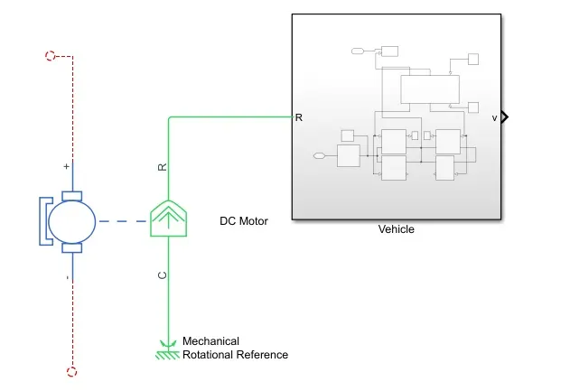
The left side of the motor represents the electrical part of the motor, whereas the right side represents the mechanical part. The mechanical part has 2 ports labelled C and R. C refers to the casing of the motor and R represents the rotation of the motor which produces the torque. The electrical part has 2 ends labelled with a positive and negative sign which represent the positive and negative terminals of the motor. Double-clicking the motor block opens the block parameters:

Electrical Torque

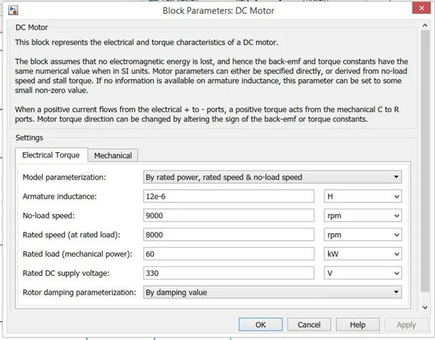
Under the "Electrical Torque" tab, we can model the electrical torque characteristics of the DC motor such as no-load speed, and rated DC supply voltage. I have used the values and settings shown in the image above.

Mechanical

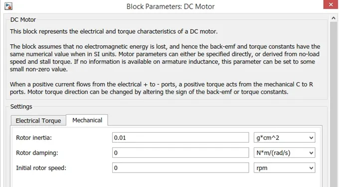
Under the "Mechanical" tab, we can model the mechanical torque characteristics such as rotor inertia and initial rotor speed. I have used the default values as shown in the image above.

After setting the DC motor block parameters, make the connections as given in the image below:

Power Converter

Power converters are needed to provide power in the necessary magnitude and form from one component to another. In the system of an EV, power converters are used to supply the motor with the required power from the battery. In this model, I have used an H-Bridge block shown below:

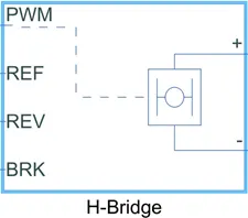
The H-Bridge block has 2 sides to it. The left side controls the voltage signals and the right side is for the terminals to provide the controlled voltage to the DC motor. The left side of the H-Bridge consists of ports which are explained below:

• PWM - This stands for Pulse Width Modulation and provides voltage pulses to the H-Bridge in either the PWM mode or Average mode.
• REF - This stands for reference.
• REV - This stands for reverse.
• BRK - This stands for brake.

Double-clicking the H-Bridge block, opens its block parameters shown in the image below:

Simulation Mode & Load Assumptions

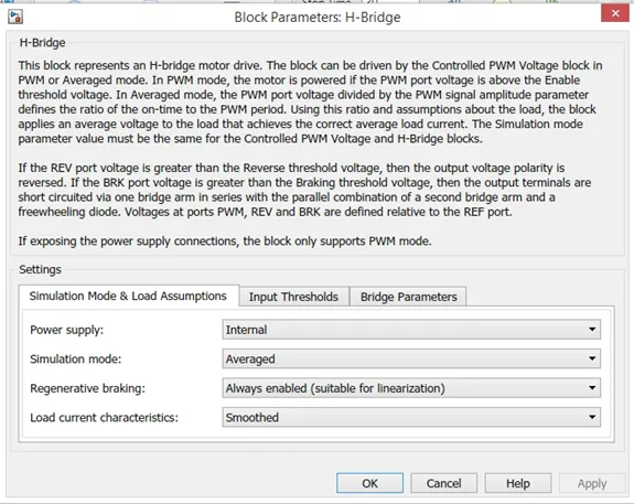
The main parameters are for the simulation mode and load assumptions of the H-Bridge. I have selected the H-Bridge to run on an "Internal" power supply with an "Averaged" simulation mode instead of the PWM mode. This is because using the PWM mode will result in significantly longer simulation times compared to using the averaged mode. I have enabled the regenerative braking mode and set the load current characteristics to the "Smoothed" option.

Input Thresholds

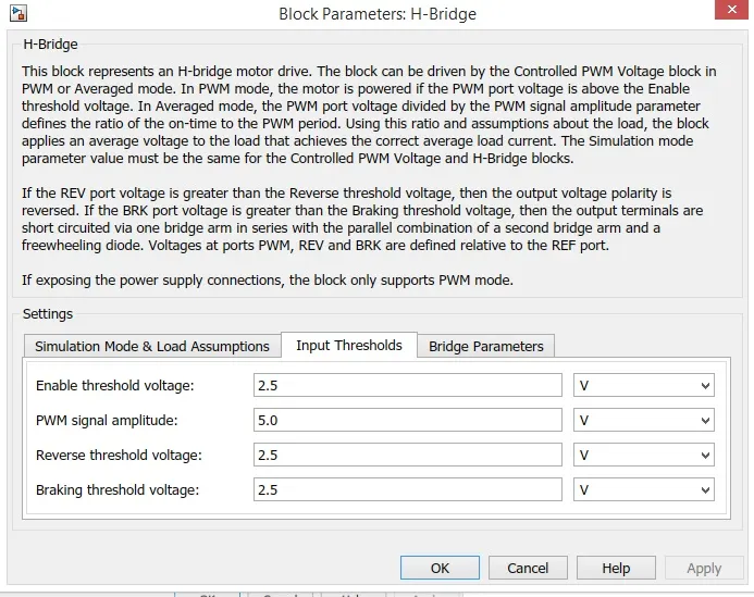
From the "Input Thresholds" tab, we can set the voltage thresholds of the 4 ports. The default values are selected.

Bridge Parameters

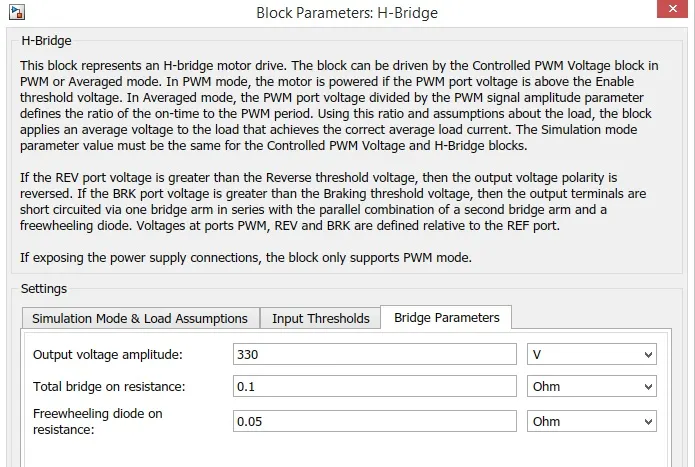
From the Bridge Parameters tab, we can modify parameters such as output voltage amplitude and total bridge on resistance. Here, only the output voltage amplitude was modified to 330V. The other parameters were kept to default.

Controlled PWM Voltage

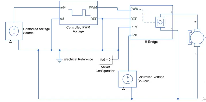
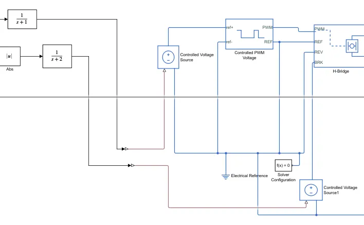
Next, I have used a 'Controlled PWM Voltage' block to provide a controlled pulse width modulated voltage to the H-Bridge block. The block will output the PWM voltage through its 'PWM' and 'REF' ports which will feed in to the same ports found on the H-Bridge block. If the pulse is low the output voltage is considered 0V whereas if the pulse is high, the output voltage will be equal to the output voltage amplitude which was set to 330V in the H-Bridge block. The pulses of voltage created by this block are dependent on the duty cycle which is the ratio of the time that the switch is ON to the time taken for 1 cycle (which is the time for which the switch is ON and OFF). The duty cycle is set by the input of the controlled PWM voltage block.

The "Controlled PWM Voltage" block is shown below:

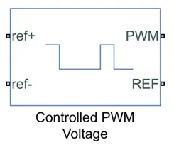
Double-clicking the block, opens the block parameters shown below:

PWM

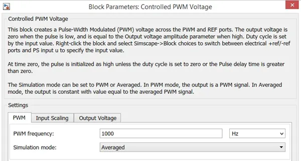
Under the "PWM" tab, I have chosen the 'Averaged' simulation mode so that the average value of the voltage pulses are generated and fed in to the H-Bridge. This will allow for quicker simulation times, just like for the H-Bridge block parameters. The remaining parameters of 'Input Scaling' and 'Output Voltage' are unchanged.

If these parameters have been applied, close the block parameter window. The connections for this block will be made later on.

Controlled Voltage Source

The input ports of the controlled PWM voltage block are still unconnected and that is because they require a controlled voltage source to provide the voltages to produce the voltage pulses to be fed in to the H-Bridge. For this, I have used the controlled voltage source block. This block is useful because it will provide the necessary voltage that is powerful enough to maintain the voltage at the output regardless of the current that passes through it.

The controlled voltage source block is shown below:

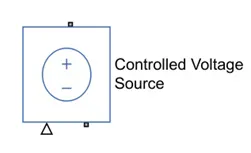
In this model, 2 controlled voltage sources have been used. One block is to provide the voltage for the acceleration of the vehicle and the other is to provide the voltage for the deceleration of the vehicle.

Electrical Reference

The electrical reference block is used to create a grounding effect for electrical circuits. Any model that uses electrical or electronics components will need to have atleast one electrical reference block in it. The electrical reference block is shown below:

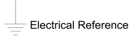
In this EV model, we are using this block for 2 occasions. The first is for to create an electrical ground between the controlled voltage source, controlled PWM voltage and the H-Bridge blocks. The second is for the battery system which will be modelled afterwards,

Solver Configuration

The solver configuration block is used to solve any necessary equations in a model and in my case, I have used them in the connection to the 'REV' port of the H-Bridge block. The solver configuration block is shown below:

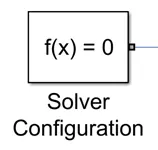
The image below shows the connections that can be made with the components discussed till this point.

Battery System

The battery system is an essential part of the EV model as it will provide the electrical power required to power the DC motor. The components of the battery system are explained below:

Battery

The battery block used is a simple one and considers only the basic parameters. The battery block is shown below:

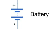
Double-clicking the battery block, opens the block parameters which is shown in the image below:

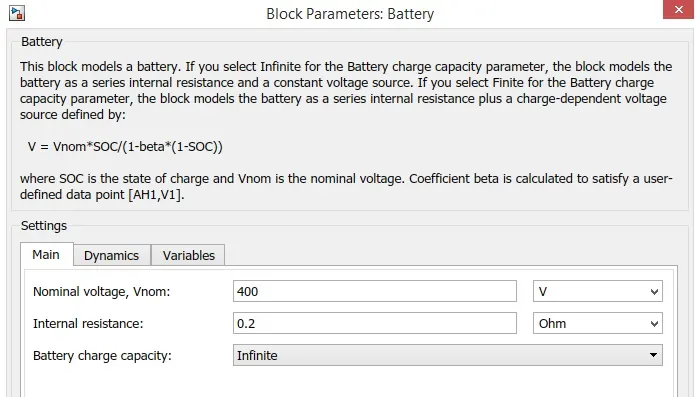
As we can see, the battery block parameters include the nominal voltage, the internal resistance and the battery charge capacity. I have used a nominal voltage of 400V, an internal resistance of 0.2 Ohms and an infinite battery charge capacity.

Controlled Current Source

The controlled current source block is a part of the battery system used in the EV model. Similar to the controlled voltage source, this block will represent an ideal current source that is powerful enough to maintain the specified current regardless of the voltage across it. The controlled current source block is shown below:

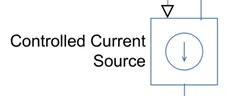
Current Sensor

The current sensor block represents an ideal current sensor and is used to convert the current measured in an electrical circuit to a physical signal that is proportional to the current. This block is used to measure the current between the battery circuit (controlled current source) and the DC motor. The current sensor block is shown below:

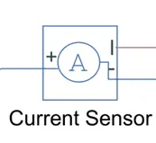
The positive and negative terminals represent the terminals across which the current sensor is inserted in to the circuit. The third port outputs the physical signal and in my model, it will send the signal to the controlled current source.

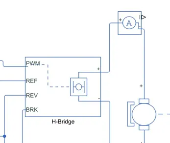
From the image above, we can see that the current sensor is embedded in between the electrical side of the DC motor and the H-Bridge. The current sensor can be connected from its physical signal port to the remaining components in the battery system including an electrical reference block. This is shown in the image below:

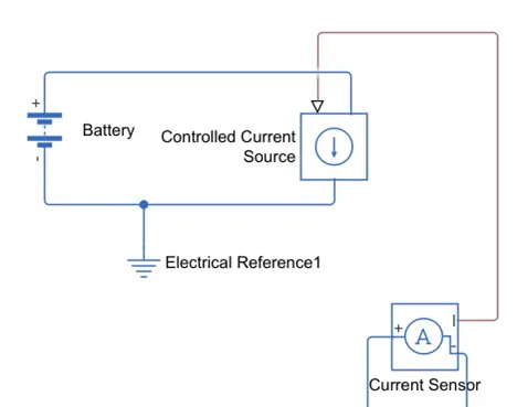
SOC & Current

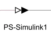
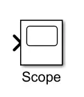
SOC stands for state of charge and it is a measurement of the available charge in a battery. When a battery is fully charged, it is considered to have a 100% charge and conversely 0% charge if fully discharged. In this EV model, I want to measure the current and the SOC of the battery as the simulation is run. For this, I have used a scope block which shows the output signal we wish to measure as a plot against time. 2 scopes have been used, one for the current and the other for the SOC. In order for this to be measured, we need to use a 'PS - Simulink converter' block. This is because the current signal is a physical one and we are measuring it as a logic signal in the SIMULINK workspace.

The PS-Simulink converter block is shown below:

The scope block is shown below:

SOC Subsystem

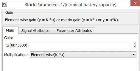
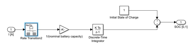
To measure the state of charge of the battery, a subsystem was created of various blocks. The first block is the 'Rate Transition' block and it is used to handle data transfer between different rates and tasks. Next, a 'Gain' block is used in order to multiply or divide the signal coming from the rate transition block. In this case, the gain block will divide the current signal with the ampere rating of the battery which has been taken as 80Ah multiplied by 3600 (seconds in an hour). This is shown in the gain block parameters below:

Then, a 'Discrete - Time Integrator' block is used to perform a discrete integration of the current signal with respect to the time. A constant block is used to represent the initial SOC of the battery. Assuming that the battery is always fully charged when performing a simulation, I have altered the constant block with a value of 1 representing 100%. Next, a 'sum' block is used to perform addition and subtraction operations. The signal from the 'discrete time integrator' block will be subtracted from the constant block representing 100% charge. These components are connected as shown below:

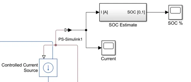
These blocks are then made in to a subsystem called 'SOC Estimate' and linked with the battery circuit using the PS-Simulink converter block. A scope block is used at the junction of the PS-Simulink converter block to plot the output signal of the current from the battery. Another scope is used to plot the output signal of the SOC from the SOC subsystem. This is shown in the image below:

Drive Control

In order to control the vehicle, we need another system that decides how the vehicle will operate. This means that data needs to be input in to this model as commands for how we desire the vehicle to operate. In addition, we need blocks that control how the vehicle will operate as a response to its instantaneous state. This system is explained below:

Drive Cycle

A drive cycle is a data set that contains velocity and time data for the purpose of modelling the motion of a vehicle. The drive cycle will be a plot of the velocity against the time and it is made to resemble typical driving conditions that a consumer may experience themselves in. For instance, they can model highway driving situations, driving in urban areas, or driving with full power etc. Drive cycles are used by automotive companies for various testing procedures such as mileage, pollution tests, and acceleration and top speed tests. There are various different drive cycles that are industry standard e.g. Urban Dynamometer Driving Schedule (UDDS), FTP 75.

In my EV model, a drive cycle is used as the reference velocity data for the longitudinal driver block to send acceleration or deceleration commands according to the drive cycle. There are 3 ways of implementing a drive cycle. One method is to create or own drive cycle with a spreadsheet of velocity data in one column and time data in another column. Another method is to use a signal builder block and create signals that represent the velocities at which the vehicle should travel and the durations for which those velocities are to be maintained. The last method is to use the industry standard drive cycles which are in - built in to the SIMULINK library. In my case, I have used an industry standard 'WOT' drive cycle. This drive cycle stands for 'Wide Open Throttle' and it models the situation where the vehicle is made to accelerate at full power and maintained at a particular speed and made to decelerate back to rest.

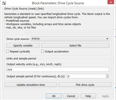
By default, the drive cycle block is set to the FTP75 drive cycle shown below:

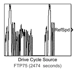
This can be modified by opening the block parameters shown below:

When the 'WOT' drive cycle is chosen, some extra parameters are made available for modification which are shown below:

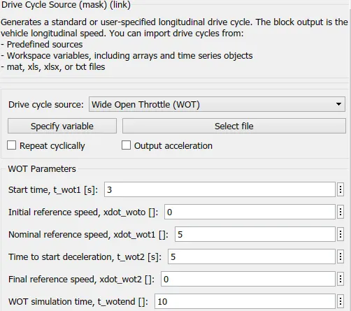
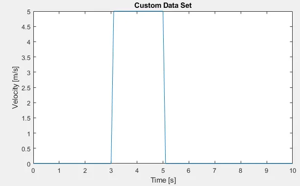
As we can see, with the 'WOT' drive cycle, we can modify the start time, time to start deceleration, and the entire duration of the drive cycle. I have used a start time of 3 seconds meaning that the vehicle will begin acceleration after 3 seconds of starting simulation. I have used a nominal reference speed of 5 m/s and this refers to the maximum speed the vehicle should achieve. I have set the deceleration to begin at t = 5 seconds and the whole cycle is set for a duration of 10 seconds. The input and output velocity units are both set to m/s.

The plot below shows the custom WOT drive cycle I have created.

Sum Block

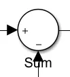
The "Sum" block is used as part of a feedback system. This system will require data from the drive cycle (command signals) and data from the vehicle body (actual speed) as well. The aim of this speed control system is to have the actual vehicle speed to match the command speed data from the drive cycle as closely as possible. The feedback system is essential to this control method because it will relay the actual speed data back for a comparison with the drive cycle data. Any difference in the data between the two is considered as an error and the sum block is used to find the difference.

This block is shown below:

Double-clicking the sum block opens the block parameters as shown below:

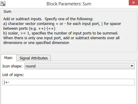
In order to find the difference between the drive cycle data and the actual speed from the vehicle block, the list of signs need to be changed to "+-".

PID Controller

The PID controller block is essential for the speed control of the EV model. The PID controller block takes the error data between the drive cycle data and the actual speed of the vehicle (from the sum block) and works to minimize this error. The PID controller block is shown below:

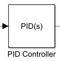
Double-clicking the block opens the block parameters shown below:

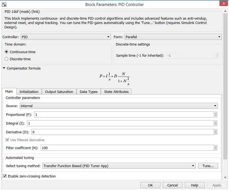
In this model, I have used the continuous-time domain PID controller. All other parameters are left as default.

Saturation Block

In order to set the acceleration and brake commands, I have used the saturation block. This block is used when we want to set limits for signals. This block is shown below:

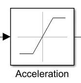
In the case of the accelerator command, I have set the limits between 0 and 1 by opening the saturation block parameters as shown below:

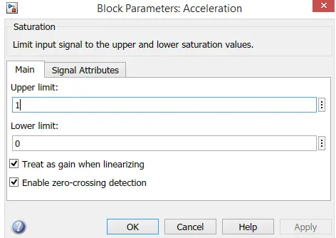
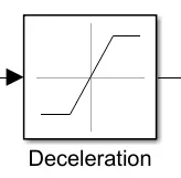
Another saturation block was used for the deceleration/brake commands which is shown below:

To create the deceleration commands, I have used a different set of limits between -1 and 0. This is shown in the image below:

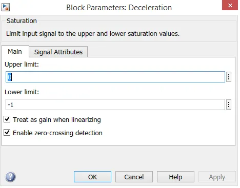
These limits ensure that there is no crossover with the acceleration commands.

Transfer Function

The transfer function block is used when we want to insert a transfer function. A transfer function is defined as the ratio of the Laplace transform of the output of a system to the input of a system. The transfer function block is shown below:

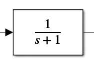
Double-clicking the block opens the block parameters as shown below:

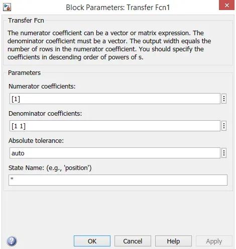
From the block parameters, we can modify the transfer function by changing the numerator and denominator coefficients. I have used the default coefficients.

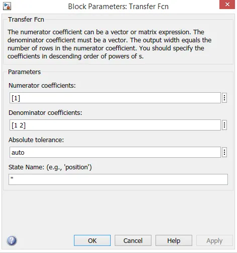
For the deceleration command, I have used another transfer function block with a slightly different transfer function. This is shown in the image below:

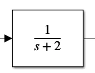
The transfer function block was modified by changing the coefficient of the denominator as shown in the image below:

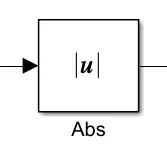
Absolute Block

An absolute block is also implemented for the deceleration command which takes the absolute value from the deceleration saturation block. This block is shown below:

With the aforementioned blocks, the control system can be made as shown in the image below:

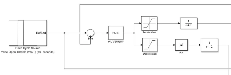
The accelerator and brake commands can be connected to the power converter as shown in the image below:

Speed Measurement

In order to measure the speed of the EV model, I needed to use the scope block once again. I modified the scope block to have 2 input ports where one port takes the output velocity signal from the vehicle subsystem block and the other port takes the output signal from the drive cycle to the reference velocity port on the longitudinal driver block. This has been done so that the scope can show us the plots of the reference velocity and the actual velocity of the vehicle to see how they compare with each other.

Distance Measurement

I have used the scope block and mathematical operator blocks to measure the distance travelled by the vehicle according to the drive cycle data. The area under a velocity time graph tells us the distance travelled by an object and so in my model. This means that the integral of the velocity with respect to time, gives us the distance travelled. So, I have implemented the integrator block to integrate the velocity signal that is output from the vehicle subsystem.

The integrator block is shown below:

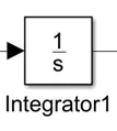
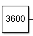
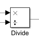
From the integrator block, I needed to use the 'Divide' block along with a 'Constant' block having a value of 3600 in order to convert the divide the integrated speed signal which is in kilometres per hour by 3600. This will give us the distance travelled in kilometres.

The constant block with a value of 3600:

The 'Divide' block:

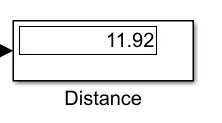
Finally, a 'Display' block is used to show the distance travelled as the simulation is run. The display block is shown below:

If these blocks have been added to the workspace, they can be connected as shown in the image below:

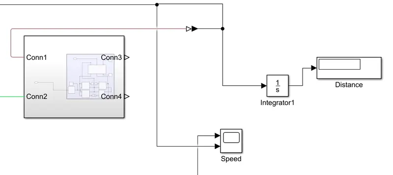
From the drive cycle block, a connection is given to the speed scope block to plot the drive cycle data during the simulation. From the speed scope block, a connection is sent back to the control system to the sum block negative port for the feedback control to occur.

Results

Without Modified Coefficients

After a simulation time of 10 seconds, the following default PID values were used:

• `K_p = 1`
• `K_i = 1`
• `K_d = 0`

The distance and speed plot shown below was obtained:

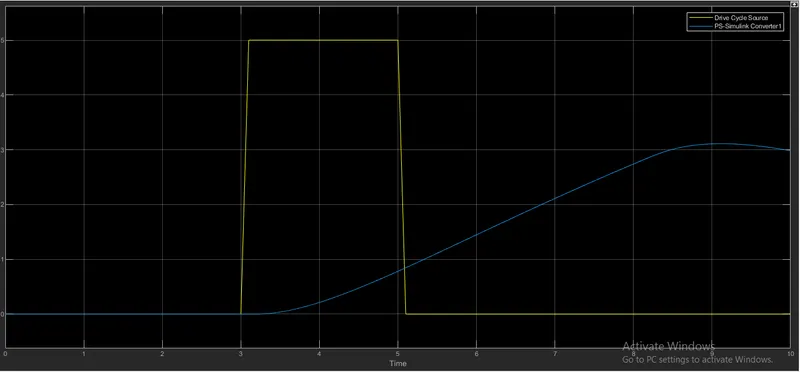
From these results, we can see that the vehicle only begins its acceleration at t = 3.4 seconds as opposed to the commanded t = 3 seconds from the drive cycle. At t = 4 seconds, the vehicle speed has increased to 0.2 m/s whereas the commanded speed from the drive cycle is 5 m/s at the same time period. By t = 5 seconds, the vehicle is meant to start its deceleration back to rest, but the vehicle is still in its acceleration phase as the speed increases to 0.8 m/s at the same time period. After t = 5 seconds, the vehicle's acceleration appears to be linear and the vehicle speed reaches its peak value of 3.1 m/s at t = 9 seconds. Immediately after, the vehicle begins deceleration and the vehicle speed drops to 3 m/s at t = 10 seconds.

For the default PID values, there appears to be a delayed response time in the actual vehicle speed. There is no overshoot and there is very minimal steady state error.

First Modification

For the same simulation time, the proportional and integral constants in the PID controller block were modified to the following:

• `K_p = 800`
• `K_i = 300`
• `K_d = 0`

For these parameters, the following speed-time plot was obtained:

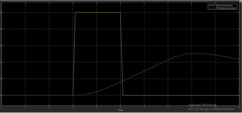
From these results, we can see the plot of the drive cycle data and the actual vehicle speed. In the actual speed of the vehicle, there is a slight delay in the acceleration of the vehicle wherein the vehicle only starts accelerating at t = 3.3 seconds instead of t = 3 seconds as seen in the drive cycle. At t = 4 seconds, the vehicle reaches 0.3 m/s which is much lower than the commanded speed of 5 m/s. By t = 5 seconds, the vehicle achieves a speed of 0.8 m/s whereas the drive cycle is still at 5 m/s and is about to begin its deceleration back to 0 m/s. The actual speed of the vehicle has a delayed response time as it is still in its acceleration stage and has not reached its peak speed value either. By t = 8 seconds, the vehicle achieves its peak speed of 2.6 m/s which is only half of the commanded peak speed. The peak speed was commanded to be maintained for 2 seconds, but the actual peak speed was not maintained and immediately begins to decrease after t = 8 seconds. At t = 9 and t = 10 seconds, the actual speed of the vehicle dropped to 2.5 m/s and 2.2 m/s respectively.

For the selected PID vales, there is a slightly quicker response time. However, compared to the default PID values, the peak speed of the vehicle was 0.5 m/s lesser in this attempt. Once again, there was no overshoot and the steady state error was minimal.

Second Modification

For the same simulation time, the following PID values were used:

• `K_p = 600`
• `K_i = 500`
• `K_d = 0`

For these parameters, the following speed-plot was obtained:

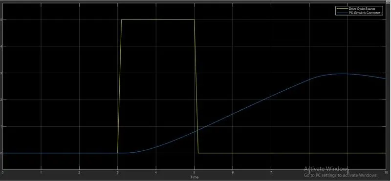
As we can see, for this attempt, the proportional constant was decreased and the integral constant was increased. The derivative constant was left as 0 as there is no overshoot in the results. From the speed-time plot, we can see that the response time of the vehicle is unchanged. Once again, the vehicle only begins its acceleration at t = 3.4 seconds just like the previous attempts. The vehicle acceleration behavior is also unchanged in that the vehicle reaches the same speeds at the same time periods as before. The vehicle reaches 0.8 m/s by t = 5 seconds and has a linear acceleration before reaching its peak speed of 3 m/s at t = 8.8 seconds. This peak speed is only maintained for 0.3 seconds before the vehicle begins its deceleration.

For these PID values, the results in the plot were shifted upwards causing the peak speed to be higher than the previous attempt. However, despite having a higher peak speed in this attempt, the peak speed was achieved quicker in the previous attempt by almost 1 second. Once again, there was no overshoot and the steady state error was minimal.

Third Modification

For the same simulation time, the following PID vales were used:

• `K_i = 550`
• `K_p = 800`
• `K_d = 0`

For these PID values, the following speed-time plot was obtained:

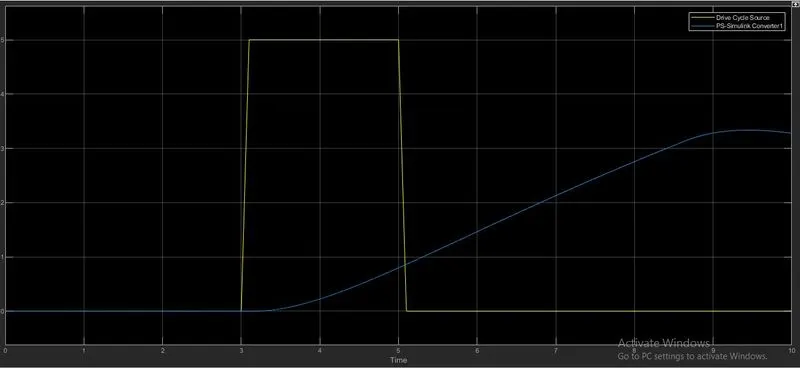
From the speed-time plot shown above, we can see that the vehicle's starting acceleration time is unchanged starting at t = 3.4 seconds once again. The vehicle reaches a speed of 0.2 m/s by t = 4 seconds and the acceleration continues in the same linear behaviour as seen in the previous attempts. While the drive cycle reference begins its deceleration back to rest at t = 5 seconds, the actual speed of the vehicle is still in its acceleration phase. The vehicle continues to accelerate and reaches a peak speed of 3.3 m/s at t = 9.2 seconds. Immediately after, the vehicle begins its deceleration phase and decelerates to 3.2 m/s at t = 10 seconds.

In this attempt, the overall speed behavior of the vehicle is unchanged. However, the peak speed was the highest compared to all other simulation attempts. There is still a delayed response time in the acceleration of the vehicle and the vehicle fails to achieve the commanded peak speed of 5 m/s. The vehicle also fails to maintain the actual peak speed for the commanded 2 seconds of time.

Conclusion

In conclusion, the vehicle speed was controlled to some extent with the implementation of the PID controller block. Since this was not a linearized system, the auto-tune feature in the PID controller block could not be used. Trial and error was performed in a few attempts to control the speed of the vehicle to match the drive cycle reference speed more closely. Despite being able to manually tune the PID controller, the vehicle speed was still unable to reach the desired peak speed value of 5 m/s from the drive cycle. In addition, the vehicle was also unable to sustain said peak speed value from the drive cycle for the desired time period of 2 seconds.

These shortcomings maybe due to the various reasons. For instance, the vehicle may be unable to achieve a value of 5 m/s due to the rolling resistance effect between the road surface and tires. Perhaps, the effect of wind resistance from the headwind also contributed to the vehicle being unable to reach the desired peak speed. If the auto-tune feature in the PID controller block was usable, it may have been possible for the vehicle to follow the drive cycle reference command more closely.