Project-1: Modelling an electric Car with Li-ion battery
Project-1: Modelling an electric Car with Li-ion battery
MATLAB model of electric car which uses lithium ion battery and suitable motor.
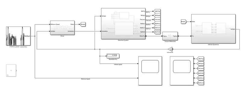
System level configurations & Model parameters
1) DRIVE CYCLE
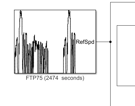
we give FTP75 drive cycle to run the model
2) DRIVER
vehicle speed control using PI controller and generate brake and accelerator commands
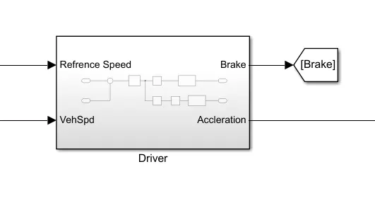
in it
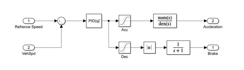
--PID
The block output is a weighted sum of the input signal, the integral of the input signal, and the derivative of the input signal. The weights are the proportional, integral, and derivative gain parameters.
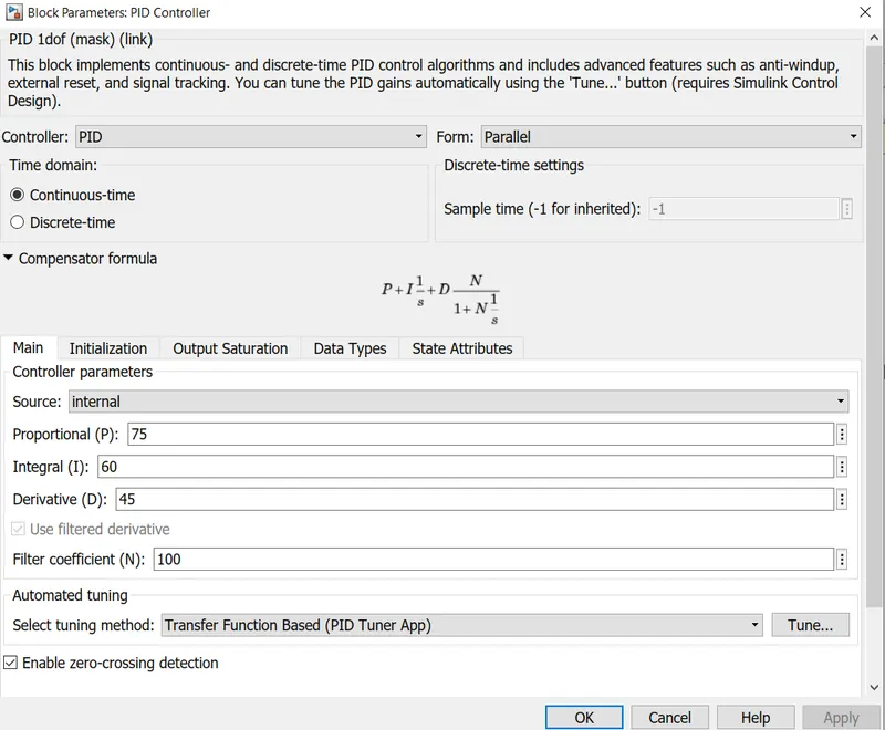
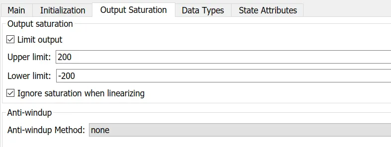
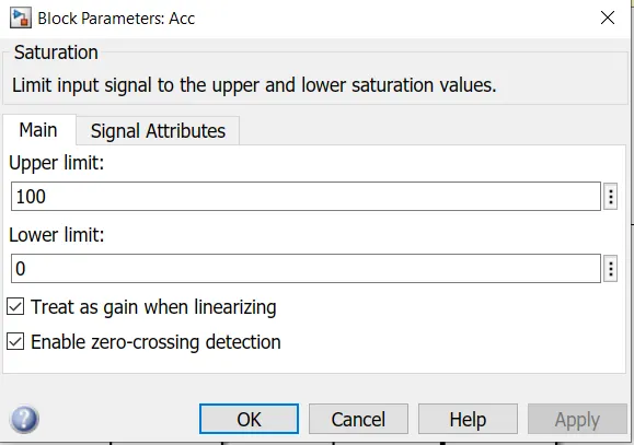
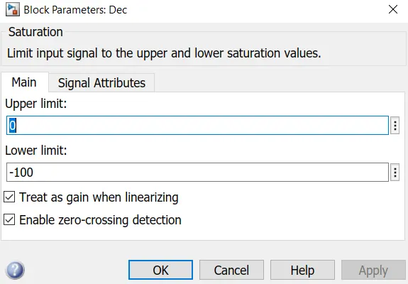
The Driver block is a controller for the vehicle, it controls the acceleration, and braking of the vehivle. The block is implemented with a PID controller which is basically the main controller in the whole drive cycle. The PID controller works as colsed loop speed control, it takes the input as a reference speed and correct the error genereted by the vehicle speeds. PID conroller is tuned for the adequate acceleration and deacceleration command itis done by limiting its output to upper and lower saturation. Separting the output of the PID to accelerate and deacceleration command we use a saturation block for each command, for acc command we use an upper saturation value and for the deaccelerate command, we use a lower saturation value.
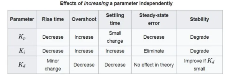
PID Gain Tuning
The PID controller coefficients are tunable either manually or automatically.
Saturation
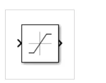
The Saturation block produces an output signal that is the value of the input signal bounded to the upper and lower saturation values. The upper and lower limits are specified by the parameters Upper limit and Lower limit.
-ACCELERATION
--DECELERATION
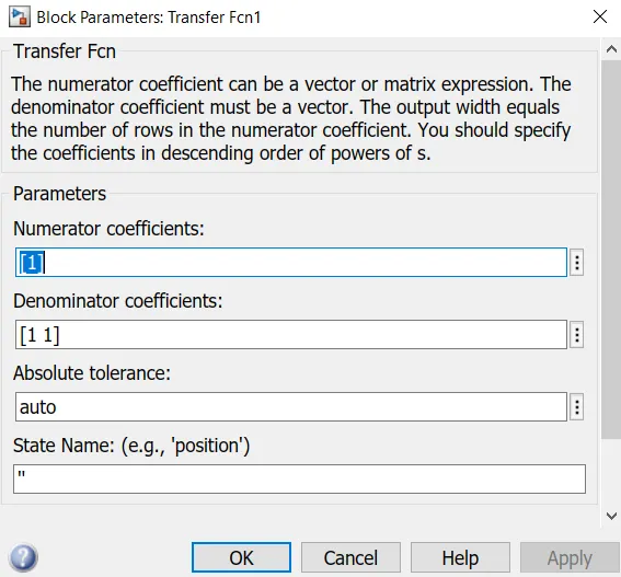
--TRANSFER FUNCTION
Transfer Function Display on the Block
The Transfer Fcn block displays the transfer function depending on how you specify the numerator and denominator parameters.
-
If you specify each parameter as an expression or a vector, the block shows the transfer function with the specified coefficients and powers of s. If you specify a variable in parentheses, the block evaluates the variable.
For example, if you specify Numerator coefficients as
[3,2,1]and Denominator coefficients as(den), wheredenis[7,5,3,1], the block looks like this: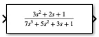
-
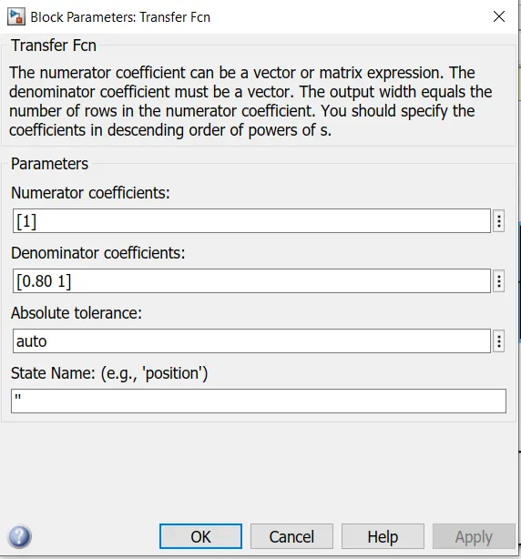
If you specify each parameter as a variable, the block shows the variable name followed by
(s).For example, if you specify Numerator coefficients as
numand Denominator coefficients asden, the block looks like this:
--Abs
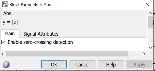
The Abs block outputs the absolute value of the input. -ve to +ve
Zero-Crossing Detection
A variable-step solver dynamically adjusts the time step size, causing it to increase when a variable is changing slowly and to decrease when the variable changes rapidly. This behavior causes the solver to take many small steps in the vicinity of a discontinuity because the variable is rapidly changing in this region. This improves accuracy but can lead to excessive simulation times.
3) ELECTRICAL SYSTEM
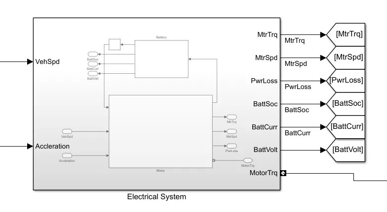
IN IT
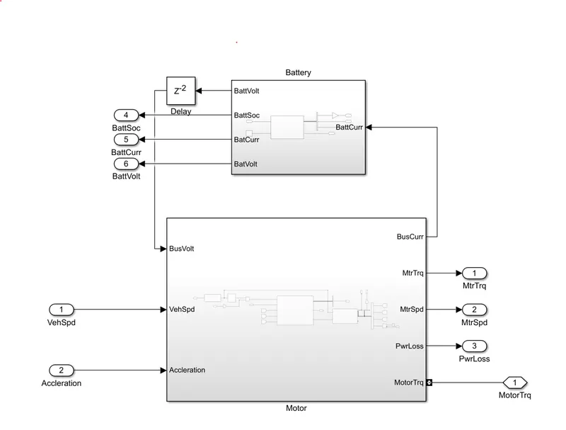
--DELAY BLOCK
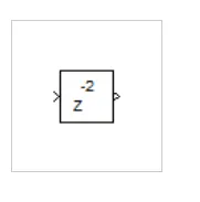
Description
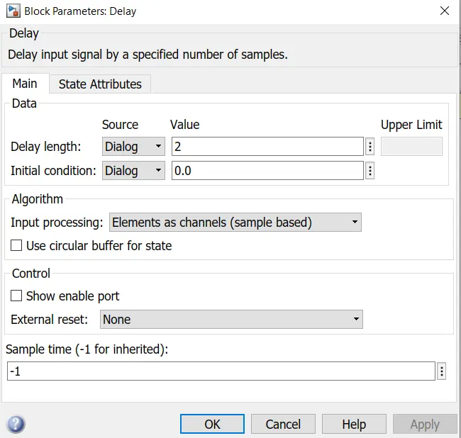
The Delay block outputs the input of the block after a delay. The block determines the delay time based on the value of the Delay length parameter. The block supports:
-
Variable delay length
-
Specification of the initial condition from an input port , etc
for more info check https://www.mathworks.com/help/simulink/slref/delay.html
>>BATTERY
The Datasheet Battery block implements a lithium-ion, lithium-polymer, or lead-acid battery that you can parameterize using manufacturer data.
To create the open-circuit voltage and internal resistance parameters that you need for the block, use the manufacturer discharge characteristics by temperature data.
To determine the battery output voltage, the block uses lookup tables for the battery open-circuit voltage and the internal resistance. The lookup tables are functions of the state-of charge (SOC) and battery temperature, characterizing the battery performance at various operating points:
Ports
Inputs
CapInit — Battery capacity
scalar
Rated battery capacity at the nominal temperature, Capbatt, in Ah.
Dependencies
To create this port, select External Input for the Initial battery capacity parameter.
BattCurr — Battery load current
scalar
Combined current flowing from the battery network, Iin, in A.
BattTemp — Battery temperature
scalar
Temperature measured at the battery housing, T, in K.
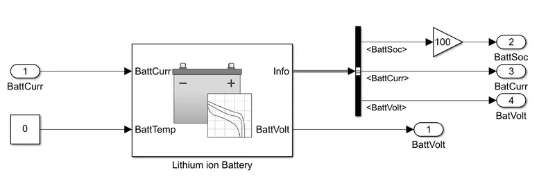
--lithium ion battery
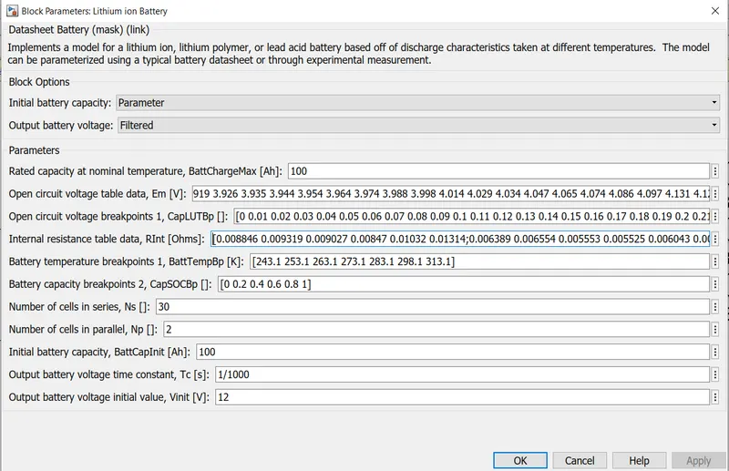
used in the system is a Datasheet battery which implements a model for the lithium-ion
battery. why most of the EV uses lithium—ion cells as a source, like any other battery because battery like a lead acid battery which required constant maintenance and monitoring, hydrogen cells which are quite bulky and expensive also capacitor banks are used as a battery pack but they have a high discharge rate and drain quickly. Hence the Lithium-Ion Battery eliminates all such disadvantages and requires fewer maintenaince and operational cost are less.
Longevity- The average lithium-ion battery life span for large capacity is more than 8 years. Safety-reduce the risk of accidents by eliminating exposures to flammable fuels able to withstand even in the high temperature without explosions.
Environment lmpact- Lithium-Ion Battery provide significaant environmental benefits over fossil fuels. With the steady increase in the electric
vehicle, we can see an immediate impact on the reduction in carbon emission.
The battery pack is packed with 30 numbers of cells in series and 2 numbers of cells in parallel each.
Rated capacity of the battery (Ah) = 100
Output Voltage = 12V
The Battery rated capacity is 100 Ah and rateed voltage is 12 volt the battery provides 1200kwh considering its charging/ discharging.
Charging of battery: If the applied current is 10 amperes, then it would be 1OOAh/1OA=1O hrs. approximately.
Discharging: Battery Ah X Battery Volt/ Applied load say, 1OOAh X 12V/100 watts = 12 hrs. (With 40% loss at the max =12 x 40/ 100 = 4.8 hrs). The
Backup will last up to 4.8 hrs.
Formula to calculate SOC = SOC(t) = SOC(t-1)+∫ [I /C Bat.dt
Where SOC(t) = State of charge at time t
SOC(t-1) = Initial state of charge
I = charge/discharge current(A)
T = time(H)
The BattCurr and the BattVolt are connected to the motor controller respectively, the batt SOC can be determined by the bus selector SOC is
scaled to 100 by using a gain block.
Parameter for Battery-
1. Battery Type = Lithium-Ion Battery
2. BattchargeMax =1OOAh
3. No of Cells in Series = 30
4. No of Cells in Parallel = 2
5. Output Battery Voltage = 12V
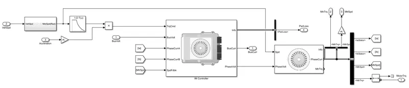
>> MOTER
>
in it

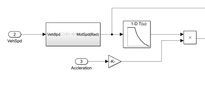
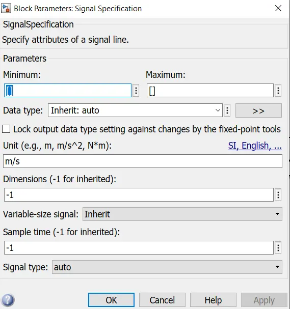
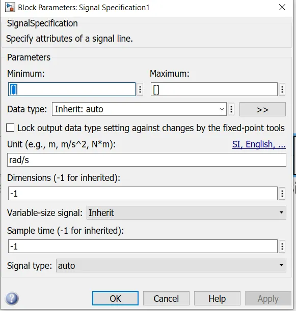
The vehicle speed in(m/s) is converted to motor speed in (rad) by the help of unit conversion and signal specification block. Taking a product of
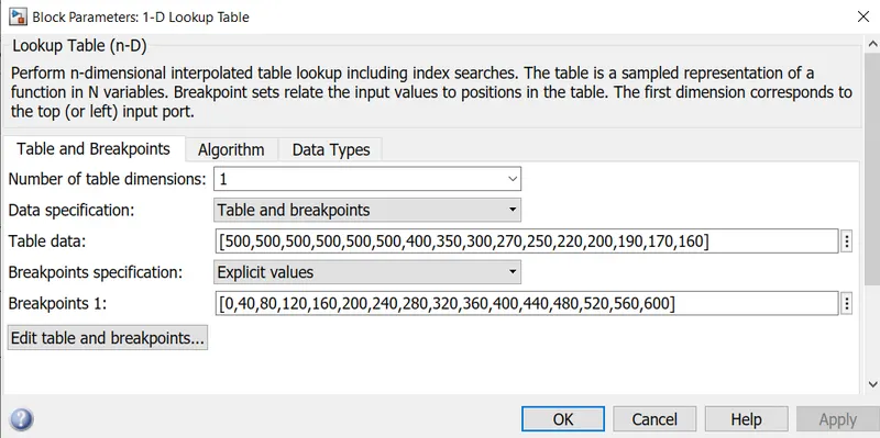
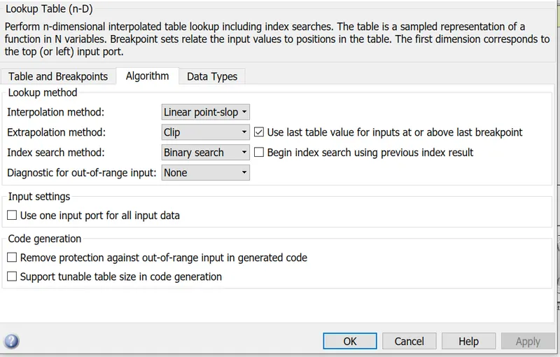
motor speed and acceleration a torque command is genereted. The lookup table takes input as vehspd in rad which is then scaled by accelerator
command and the product of two is implemented as a torque command.
--LOOKUPTABLE
Use blocks from the Lookup Tables library to model nonlinearity. Lookup table blocks use arrays of data to map input values to output values, approximating mathematical functions. To approximate a function in N variables, use the n-D Lookup Table block
| 1-D Lookup Table | Approximate one-dimensional function |
| 2-D Lookup Table | Approximate two-dimensional function |
etc
1-D Lookup Table
Supported Block Operations
The 1-D, 2-D, and n-D Lookup Table blocks evaluate a sampled representation of a function in N variables
y=F(x1,x2,x3,...,xN)
for more info --https://www.mathworks.com/help/simulink/slref/1dlookuptable.html
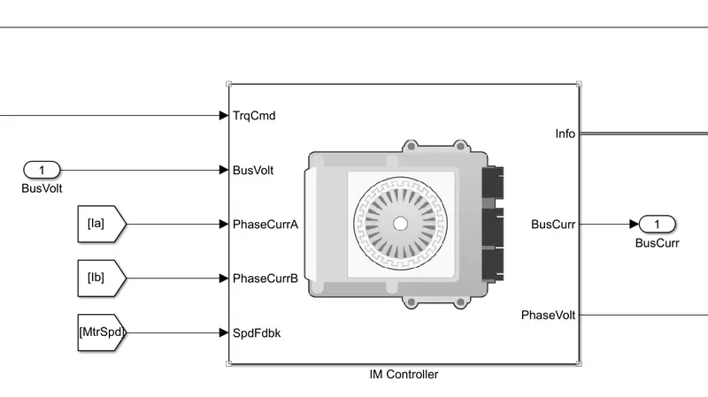
>IM CONTROLLER
Description
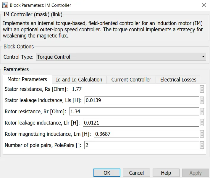
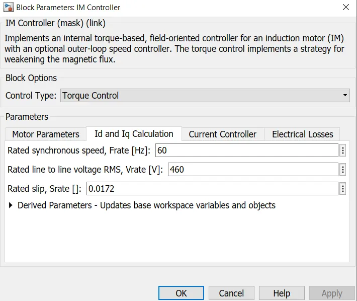
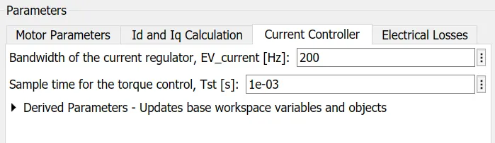
The IM Controller block implements an internal torque-based, field-oriented controller for an induction motor (IM) with an optional outer-loop speed controller. The torque control implements a strategy to control the motor flux. You can specify either speed or torque control. The IM Controller implements equations for speed control, torque determination, regulators, transforms, and motors. The figure illustrates the information flow in the block.
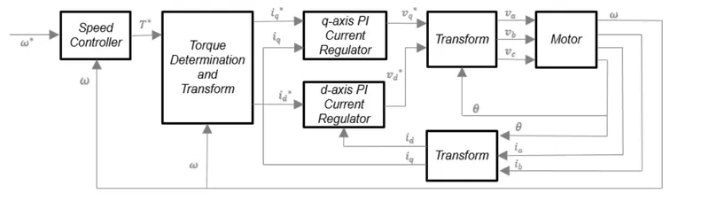
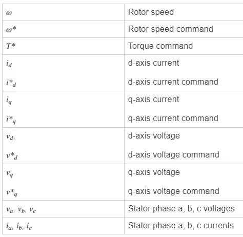
Speed Controller
To implement the speed controller, select the Control Type parameter Speed Control. If you select the Control Type parameter Torque Control, the block does not implement the speed controller.
The speed controller determines the torque command by implementing a state filter, and calculating the feedforward and feedback commands. If you do not implement the speed controller, input a torque command to the IM Controller block.
The corresponding phases (A,B) is connected to the motor controller the speed of the motor is constantly regulated by its controller closed loop
speed control (Sdedk port).
Ports
Input
SpdReq — Rotor mechanical speed command
scalar
Rotor mechanical speed command, ω*m, in rad/s.
Dependencies
To create this port, select Speed Control for the Control Type parameter.
BusVolt — DC bus voltage
scalar
DC bus voltage vbus, in V.
PhaseCurrA — Current
scalar
Stator current phase a, ia, in A.
PhaseCurrB — Current
scalar
Stator current phase b, ib, in A.
SpdFdbk — Rotor mechanical speed
scalar
Rotor mechanical speed, ωm, in rad/s.
Info — Bus signal
bus
Bus signal containing these block calculations.
| Signal | Description | Units |
|---|---|---|
|
|
Source power |
W |
|
|
Load power |
W |
|
|
Power loss |
W |
|
|
Estimated motor torque |
N·m |
BusCurr — Bus current
scalar
Estimated DC bus current, ibus, in A.
PhaseVolt — Stator terminal voltages
array
Stator terminal voltages, Va, Vb, and Vc, in V.
https://www.mathworks.com/help/autoblks/ref/imcontroller.html
> INDUCTION MOTER
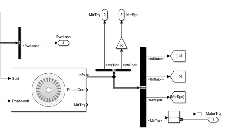
Description
The Induction Motor block implements a three-phase induction motor. The block uses the three-phase input voltages to regulate the individual phase currents, allowing control of the motor torque or speed.
By default, the block sets the Simulation Type parameter to Continuous to use a continuous sample time during simulation. If you want to generate code for fixed-step double- and single-precision targets, considering setting the parameter to Discrete. Then specify a Sample Time, Ts parameter.
Ports
Input
LdTrq — Rotor shaft torque
scalar
Rotor shaft input torque, Tm, in N·m.
Dependencies
To create this port, select Torque for the Port configuration parameter.
Spd — Rotor shaft speed
scalar
Angular velocity of the rotor, ωm, in rad/s.
Dependencies
To create this port, select Speed for the Port configuration parameter.
PhaseVolt — Stator terminal voltages
1-by-3 array
Stator terminal voltages, Va, Vb, and Vc, in V.
Output
Info — Bus signal
bus
PhaseCurr — Phase a, b, c current
1-by-3 array
Phase a, b, c current, ia, ib, and ic, in A.
MtrTrq — Motor torque
scalar
Motor torque, Tmtr, in N·m.
Dependencies
To create this port, select Speed for the Port configuration parameter.
MtrSpd — Motor speed
scalar
Angular speed of the motor, ωmtr, in rad/s.
Dependencies
To create this port, select Torque for the Port configuration parameter.
--INDUCTION MOTER BLOCK
>>VEHICLE DYNAMICS
>TORQUE DIFFERENTIAL
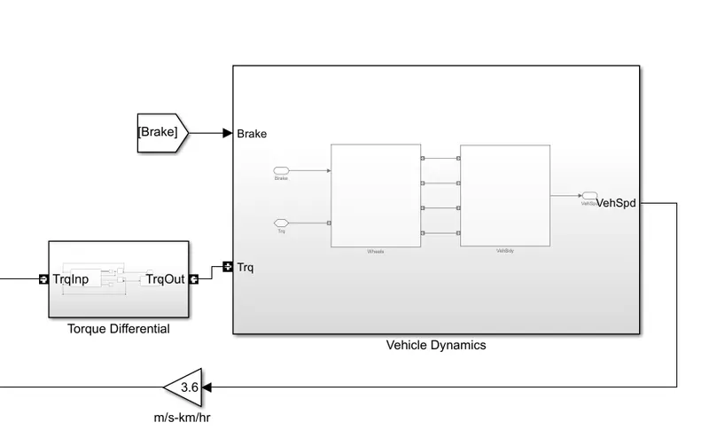
Description
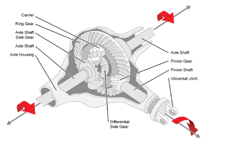
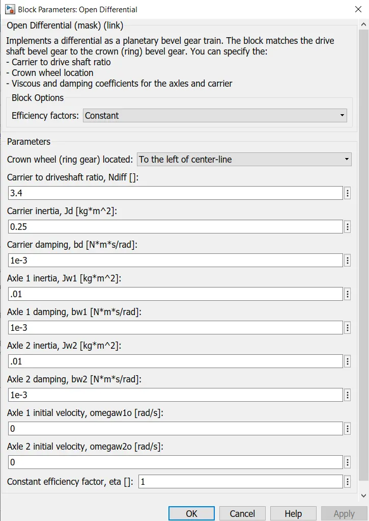
The Open Differential block implements a differential as a planetary bevel gear train. The block matches the driveshaft bevel gear to the crown (ring) bevel gear. You can specify:
-
Carrier-to-driveshaft ratio
-
Crown wheel location
-
Viscous and damping coefficients for the axles and carrier
Use the Open Differential block to:
-
Dynamically couple the post-transmission driveshaft to the wheel axles or universal joints
-
Model simplified or older drivetrains when optimal traction control does not require passive or active torque vectoring
-
Model mechanical power splitting in generic gearbox and drive line scenarios
The block uses a coordinate system that produces positive tire and vehicle motion for standard engine, transmission, and differential configurations. The arrows indicate positive motion.
Ports
Inputs
DriveshftTrq — Torque
scalar
Applied input torque, typically from the engine crankshaft, in N·m.
Axl1Trq — Torque
scalar
Axle 1 torque, T1, in N·m.
Axl2Trq — Torque
scalar
Axle 2 torque, T2, in N·m.
Temp — Temperature
scalar
Temperature, in K.
Dependencies
To enable this port:
-
Set Efficiency factors to
Driveshaft torque, speed and temperature. -
Select Input temperature.
Output
Info — Bus signal
bus
DriveshftSpd — Angular speed
scalar
Driveshaft angular speed, ωd, in rad/s.
Axl1Spd — Angular speed
scalar
Axle 1 angular speed, ω1, in rad/s.
Axl2Spd — Angular speed
scalar
Axle 2 angular speed, ω2, in rad/s.
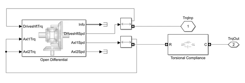
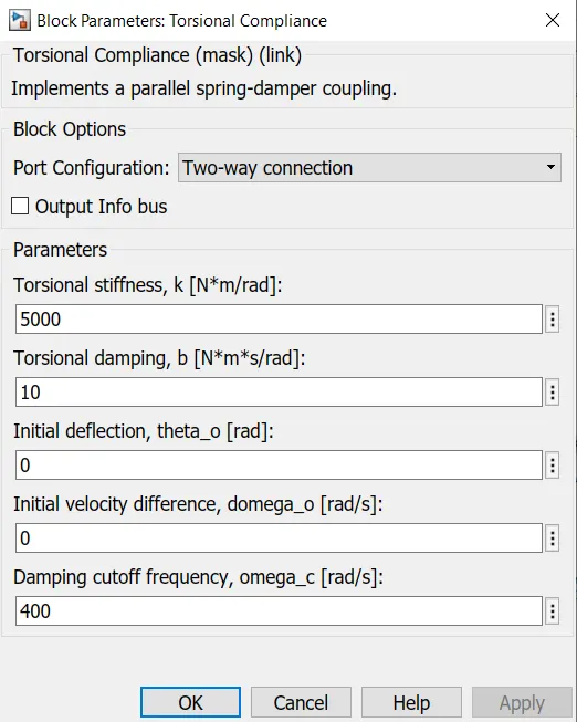
The Torsional Compliance block implements a parallel spring-damper to couple two rotating driveshafts. The block uses the driveshaft angular velocities, torsional stiffness, and torsional damping to determine the torques.
>>IN VEHICLE DYNAMICS
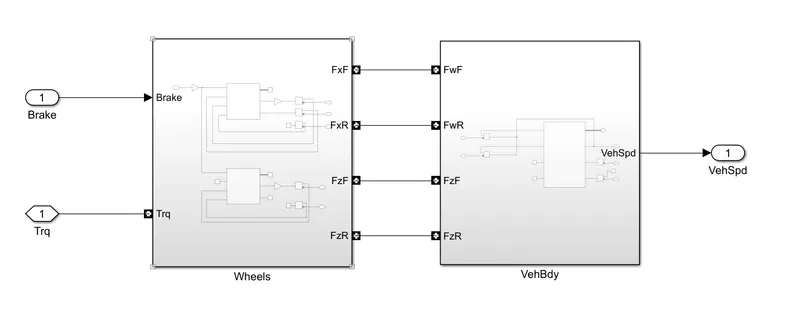
>WHEELS
The Longitudinal Wheel block implements the longitudinal behavior of an ideal wheel. You can specify the longitudinal force and rolling resistance calculation method, and brake type. Use the block in driveline and longitudinal vehicle simulations where low frequency tire-road and braking forces are required to determine vehicle acceleration, braking, and wheel-rolling resistance. For example, you can use the block to determine the torque and power requirements for a specified drive cycle or braking event. The block is not suitable for applications that require combined lateral slip.
There are four types of Longitudinal Wheel blocks. Each block implements a different brake type.
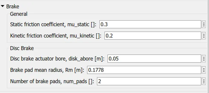
one of it is Longitudinal Wheel - Disc Brake
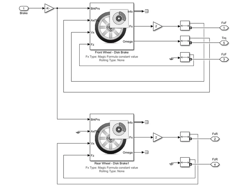
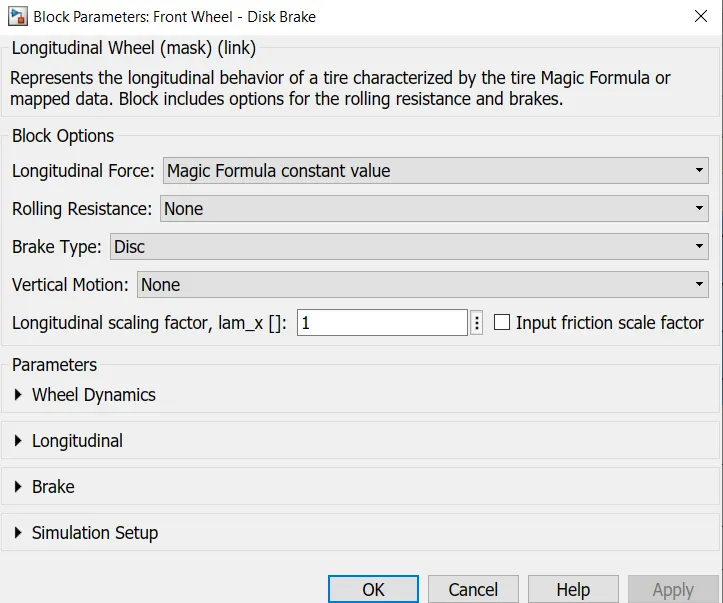
The wheels used in this vehicle are longitudnal wheels have brakes of disc type brakes have great stopping power and cause less wear and tear and provide precises braking. This block implements the longitudnal behaviour of actual wheels.
This vehicle is front wheeled drive hence the axle torque is connected to the front of the wheels and the axle of the rear wheel is Grounded.
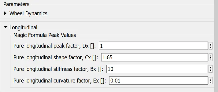
The longitudnal forces of the tires are set to magic formula constant the magic formula is a separate from of a characteristics function of stiffness, shape, peak and curvature. (BCDE)
he Magic Formula is a specific form for the tire characteristic function, characterized by four dimensionless coefficients, B, C, D, and E, or stiffness, shape, peak, and curvature:
Magic Formula is given as (FF : f(k2, Fz) : FZD sin(C'tan — 1[{BK — EIBK — tan — 1(Bk)]}])
The Brake input command for the front and rear wheels are connected commonly as one input port. Omega is the angular velocity of the wheels in
the y-axis, hence this force is considered as torque input to the wheels.
https://www.mathworks.com/help/autoblks/ref/longitudinalwheel.html#responsive_offcanvas
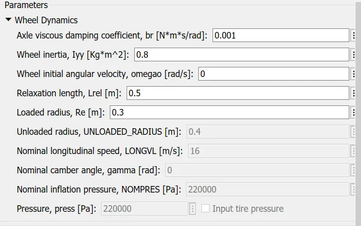
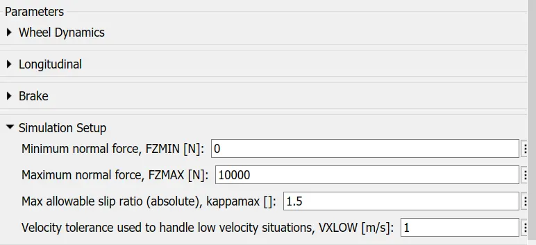
Parameters for Wheels—
1. Wheels Inertia = O.8kg*m"2
2. Wheel Radius = 0.3m
3. Tire Pressure = 220000
4. Brake Pad Radius = 0.1778m
> IN VEHICLE BODY
Description
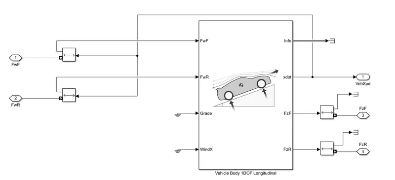
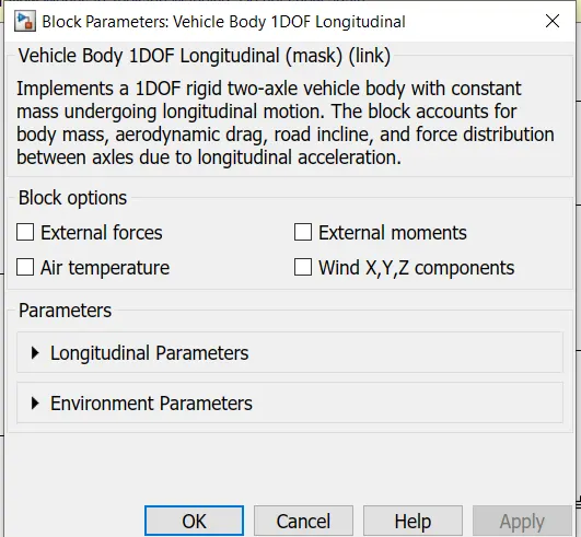
The Vehicle Body 1DOF Longitudinal block implements a one degree-of-freedom (1DOF) rigid vehicle body with constant mass undergoing longitudinal (that is, forward and reverse) motion. Use the block:
-
In powertrain and fuel economy studies to represent the vehicle inertial and drag loads when weight transfer from vertical and pitch motions are negligible.
-
To determine the engine torque and power required for the vehicle to follow a specified drive cycle.
You can select block options to create input ports for external forces, moments, air temperature, and wind speed.
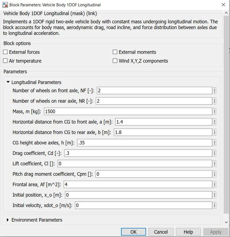
In this model vehicle body (1DOF) longitudnal block is implemented. This bolck helps us to determine the vehicle inertia and drag load. There are mainly two forces acting on the wheels which are Longitudnal Force and Normal Force. These forces act on the rear and front of the wheels, the longitudnal forces on rear and front is given by (FwF & FwR). Whereas the normal forces are given by (FzF & FzR). This forces is connected to the respective axle of the wheels.
The Vehicle Body consist of grade and wind input ports which can be used to simulate slope and wind drag but this port are been grounded to minimize the complexity of the model. The Xdot output port is a longitudnal force in the X-Axis which acts as the velocity/speed of the vehicle in
m/s.
Ports
Input
FwF — Total longitudinal force on front axle
scalar
Longitudinal force on the front axle, Fxf, along vehicle-fixed x-axis, in N.
FwR — Total longitudinal force on rear axle
scalar
Longitudinal force on the rear axle, FwR, along vehicle-fixed x-axis, in N.
Grade — Road grade angle
scalar
Road grade angle, γ, in deg.
WindX — Longitudinal wind speed
scalar
Longitudinal wind speed, Ww, along earth-fixed X-axis, in m/s.
Dependencies
To enable this port, clear Wind X,Y,Z components.
WindXYZ — Wind speed
array
Wind speed, Ww, WwY, WwZ along inertial X-, Y-, and Z-axes, in m/s. Signal vector dimensions are [1x3] or [3x1].
Dependencies
To enable this port, select Wind X,Y,Z components.
AirTemp — Ambient air temperature
scalar
Ambient air temperature, Tair, in K. Considering this option if you want to vary the temperature during run-time.
Dependencies
To enable this port, select Air temperature.
Output
Info — Bus signal
bus
xdot — Vehicle body longitudinal velocity
scalar
Vehicle body longitudinal velocity along the earth-fixed reference frame X-axis, in m/s.
FzF — Front axle normal force
scalar
Normal load force on the front axle, Fzf, along vehicle-fixed z-axis, in N.
FzR — Rear axle normal force
scalar
Normal force on rear axle, Fzr, along the vehicle-fixed z-axis, in N.
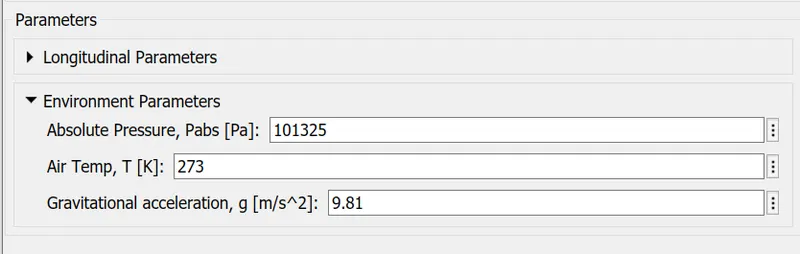
Parameters of the Vehicle Body--
>> SCOPE's
1) RESULTS
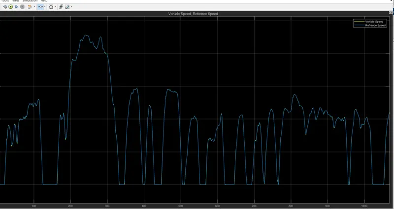
VEHICLE SPEED VS REFERENCE SPEED NEARLY SAME
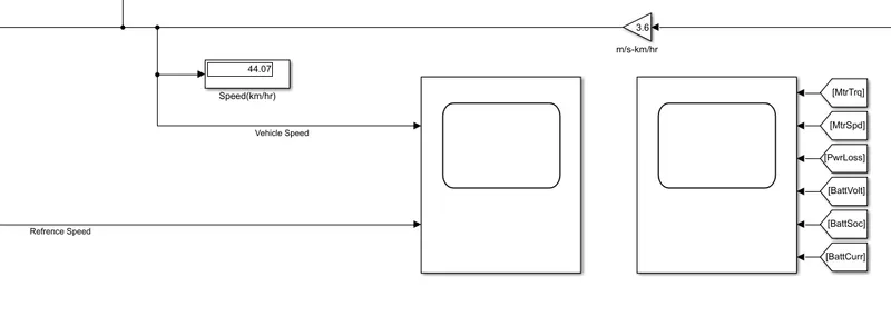
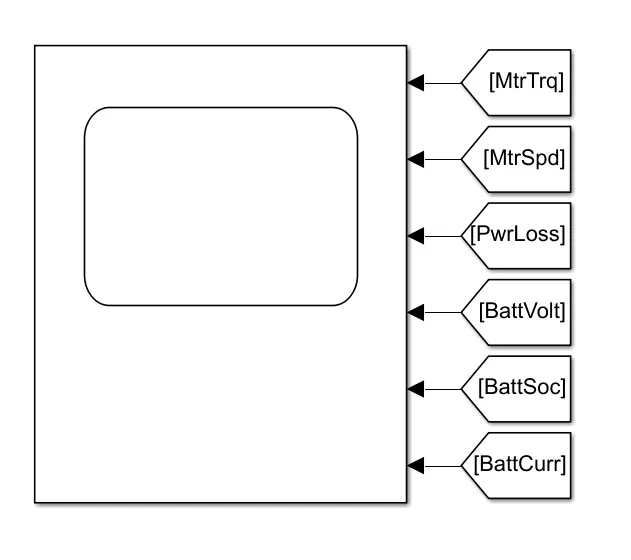
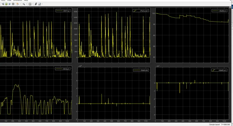
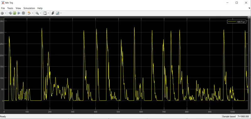
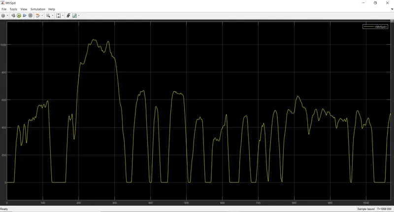
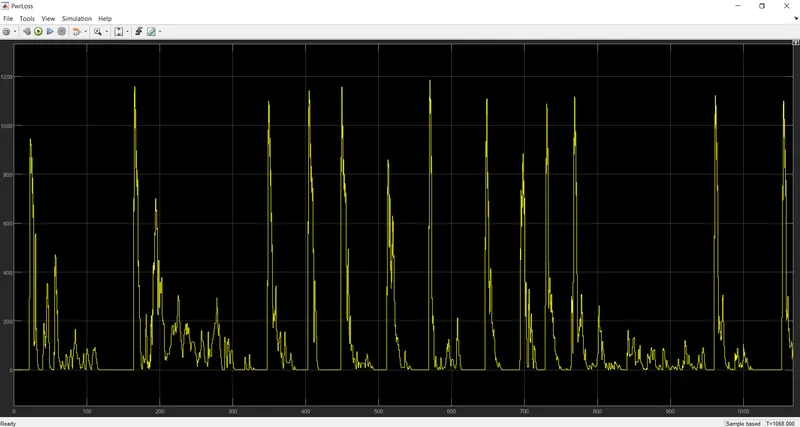
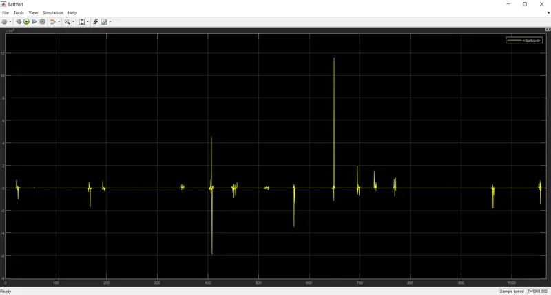
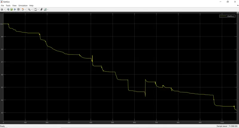
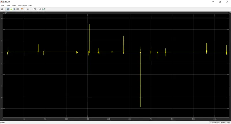
The run for about 1068 sec and we have obtaoned result shown below. There are 6 individual graphs showing the result for motor and the bateery in this result, we see that a max torque of about 320Nm was obtained and a max speed of the motor was about 1100rpm at 44kmph. The graph of the battery SOC shows a linear and a slow discharge rate, The Result for the Vehicle speed and reference speed is shown below
Mtr Trq
MtrSpd
PwrLoss
BattVolt
BattSoc
BattCurr
CNCLUSION-
we Create a MATLAB model of electric car which uses lithium ion battery with suitable motor. by using suitable blocks from Simscape or Powertrain block set. and we Implement the vehicle speed control using PI controller and generate brake and accelerator commands. we have seen System level configurations, Model parameters, the model run as per our reference input given with less error in it due to pid controller