Project 1 - FULL HYDRO case set up (PFI)
AIM:
1) To setup the case and run the full hydrodynamic simulation of a PFI Engine.
2) To find out the compression ratio of this PFI Engine.
3) To calculate the combustion efficiency of this engine.
4) To determine the torque and power of the engine using the engine performance calculator.
5) To understand significance of Ca10, Ca50 and Ca90.
6) To understand the need of wall heat transfer model.
INTRODUCTION AND THEORY:
PFI Engine: Port fuel injected internal combustion engine or PFI IC Engine is a type of IC engine where the fuel is injected into the intake port so that it is mixed with the incoming air. The fuel injectors in PFI engines are typically mounted in the intake manifold and the air/fuel mixture is pulled into the cylinder head as the intake valve opens.
Spray modelling:
Spraying of the fuel inside the cylinder from the intake port to the cylinder is done every cycle during the operation of a PFI Engine. This phenomenon can be simulated accurately by using suitable equations but the drawback is that the simulation is too large to fit it as a step in simulating the PFI engine. So, approximate methods to calculate the spray motion and its relevant parameters has been made and these are the Spray models.
The spray models that converge uses are:
For gaseous spray: Eulerian solver
For liquid spray: Lagrangian solver to model to model discrete models and Eulerian solver to model the continuous fluid domain.
Liquid spray is made up of parcels and a parcel is a collection of identical drops.The parcel entirely represents statistically the entire spray field. This type of spray modelling is called Lagrangian spray modelling or discrete phase modelling.
The information needs to be tranferred from Eulerian gas phase to the lagrangian phase and this is done by using aditional models. For example, the heat, momentum and mass transfer occur between the discrete and continuous phases through source terms in the transport equations.
Converge solves radius, velocity etc per-parcel basis.
Parcels undergo several physical processes. They are:
1) Primary breakup
2) Secondary breakup
3) Drag drop
4) Collision and coalescence
5) Turbulent dispersion
6) Evaporation
Below figure shows the spray and its physical models:
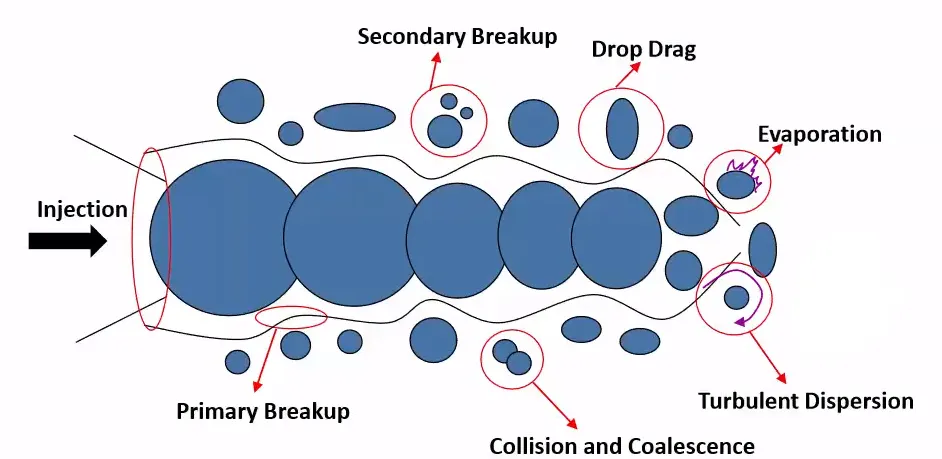
1) Primary breakup: When the fuel injection takes place, due to the interaction of liquid with the surrounding air, there is going to be a drag force which causes disturbances in the length of the liquid spray. If the disturbances ar elarge enough then at some parts of the spray, the spray breaks into tiny parcels. This phenomenon of the spray breaking up into tiny parcels is called Primary breakup.
2) Secondary breakup: After primary breakup, the tiny parcels can further breakup into even smaller parcels. This phenomenon is called secondary breakup.
3) Drop drag: The drops as they interact with the ambient air their shaes get affected which would result in a faster or slower vaporisation. This is called as drop drag.
4) Collision and coalescence: This phenomenon refers to the collision among the tiny parcels as well as merging of the tiny parcels after collision.
5) Turbulent dispersion: The turbulent dispersion takes into account the of fluctuating velocity in the gas phase on the drop.
6) Evaporation: This phenomenon refers to the reduction in size of the tiny parcels due to the conversion of liquid into vapour.
Spray modelling in converge:
General:
Parcel distribution:
There are two options in the drop down list:
i) Cluster parcels near cone center.
ii) Distribute parcels evenly throughout the cone.
The suitable option is selected according to the requirement.
Evaporation model:
To calculate the drop radius rate of change, there are two models available as options in converge.
a) Frossling model
b) Chiang model
Evaporation source:
There are three options.
i) Source specified species: All the specified parcels are evaporated to specified species.
ii) Source all composite parcel species: If composites are defined, then the multi-component liquid species evaporate into composite species.
If composites are not defined, then the multi-component species evaporate into base species.
iii) Source all base parcel species: The multi-component species evaporate into base species whether or composites are defined or not.
Maximum radius for ODE droplet heating:
This parameter controls the uniformity of drop temperature.
For drops having larger radius, the temperature inside the drop and the temperature outside the drop is different.
If the drop radius is more than the maximum value then Converge will assume a radially varying temperature distribution.
If the drop radius is less than the maximum value then converge will assume a unifor temperature distribution.
Spray penetration:
Converge writes the liquid and vapour penetration lengths at each specified output interval in the penetration tab.
For the liquid penetration length the liquid fuel mass fraction is provided.
The liquid penetration length is the distance encompassing the calculated penetrated spray mass.
The penetrated spray mass is calculated by multiplying the mass fraction by the total liquid mass in the domain.
Liquid penetration length is not calculated along the spray axis of the nozzle but along the injector axis.
Vapour penetration length is calculated as follows:
1) The fuel vapour mass fraction in each cell inside the spray cone is calculated.
2) For each cell that meets the following two conditions, the distanc efrom the centre of the nozzle to the centre of the cell is calculated.
The two conditions are:
a) The fuel vapour mass fraction exceeds the user specified value of fuel vapour mass fraction.
b) The cell size does not exceed the user specified Bin size. The recommended bin size is atleast twice the number of cells in the spray cone.
The vapour penetration length is the maximum distance calculated in the second step.
Mass diffusivity constants:
D is the mass diffusivity of liquid vapour in air
`rho_(gas)D = 1.293D_o(T_(gas)/273)^(n_0-1)`
The related connstants `D_o and n_o` are set.
From the drop down menu, select the default `D_o and n_o` values for common fuels.
Collision/Coalescence:
Options for drop collisions:
i) No collision
ii) O'Rourke numerical algorithm
iii) NTC numerical algorithm
Based upon the type of engine, one option can work better than the other.
Collision/Coalescence outcome options:
i) O'Rourke collision outcomes
ii) Post collision outcomes.
Collision mesh:
In a typical spray simulation, parcels can collide with parcels only in the same cell, which can lead to grid sensitivity.
Converge has an adaptive collisioin mesh option to reduce grid sensitivity.
If the collision mesh option is checked, the parcels can collide across grid cells.
This feature is independent of the gas phase grid and used only for collision calculations.
Drop drag:
There are several options for drop drag.
i) No drop drag
ii) Spherical drop drag: The drag co-efficient calculation assumes the drops are perfect spheres.
iii) Dynamic drag model: Th edrag co-efficient calculations accounts for variations in the drop shape.
This model invokes the TAB model to determine the drop distortion.
Drop/wall interaction:
There are several drop/wall interaction models.
i) Rebound/slide: Drops can either rebound or slide after impingement.
ii) Wall film: Drop actions are calculated based on particle based quantities or film based quantities.
iii) Vanish: Drops vanish after hitting a WALL boundary.
Combustion Modelling:
Combustion process provides energy for the engine.
Converge provides varieties of ways to simulate the combustion whic takes place in an IC engine. There is a detailed approach called detailed chemistry solver (SAGE) and there are some combustion models with some approximations.
The only problem with the detailed chemistry approach is that it is very slow.
SAGE model:
SAGE detailed chemistry solver uses local conditions to calculate reaction rates based on principles of chemical kinetics.
It solves detailed chemical kinetics during combustion and determines kinetically limited phenomena such as engine knock and emissions.
The rate of change of species concentration are calculated using the Arrhenius rate law equation.
It reads a chemical reaction mechanism in CHEMKIN format and solves ODEs to find the reaction rates.
It couples with the transport solver through source terms in the species transport equations.
It parallelizes independent of the flow solver.
Each time step the chemistry solver calculates the new species mass fractions immediately prior to solving the transport equations.
The change in the species mass fractions is treated as a source
`(del(barrhoY_m))/(delt) + (del(barrhou_jY_m))/(delx_j) = del/(delx_j)(barrhoD_t(delY_m)/(delx_j)) + omega_m`
Where `omega_m` is the source term.
The system of ordinary reactions is is solved using CVODES (general ODE solver).
The elementary reactions in the mech.dat are in Arrhenius format.
The forward reaction rate is given by:
`k_(f) = A_r*T^b* e^(-E_r/(R_ut))`
Where `A_r` is the pre-exponential factor
b is the temperature exponent
`E_r` is the activation energy
R is the universal gas constant
The reverse reaction rate can be user- specified or calculated from the equilibrium constant which is determined from properties in therm.dat.
SAGE model in converge:
Although this method is a time consuming, converge provides the following options to speed up this method.
i) Increase the minimum cell temperature and minimum Hydro carbon species mole fraction to reduce the number of cells in which the combustion calculations are performed.
ii) Use start time and stop time to limit SAGE to specific time intervals.
iii) Limit SAGE to specific regions.
iv) Set the resolve option to "Only resolve if temperature changes by specified value".
a) To maintain solution accuracy the re-solve temperature less than or equal to 2k is recommended.
v) Check "analytical jacobian" to pass an analytically calculated jacobian to the solver.
a) This option is recommende for reactions in arrhenius form.
vi) The Multizone models reduces the number of SAGE calculations by
a)grouping cells into bins.
Bins are created based on two or more variables such as equivalence ratio, temperature, pressure,reaction ratio and cube root of the mass fractions of the specified species.
b) calculating average quantities
c) Invoking the SAGE solver once per bin instead of once per cell.
d) Mapping th esolved quantities to all cells in the bin.
vii) "Conserve `NO_x` during species remap" is checked to allow mapping based on nitrogen atomsand thus improve `NO_x` emissions.
FULL HYDRO CASE SETUP:
Surface preparation, boundary flagging and no hydro case setup for the PFI Engine has been done and their procedures can be found in the link given below.
By using the no hydro setup, here are the steps to setup the full hydro case of a PFI internal combustion engine.
Materials:
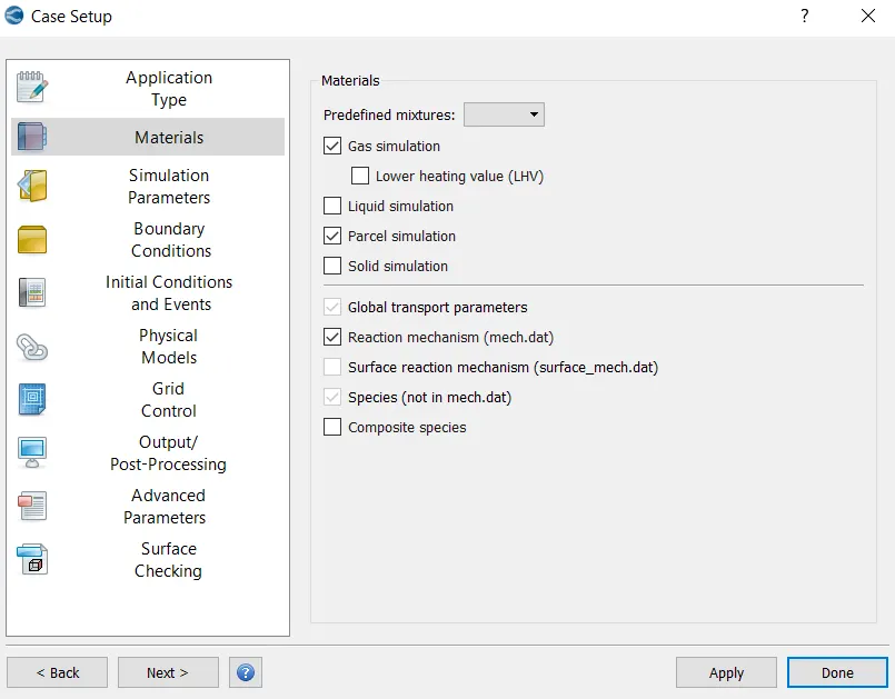
In the materials section "Parcel simulation" is checked.
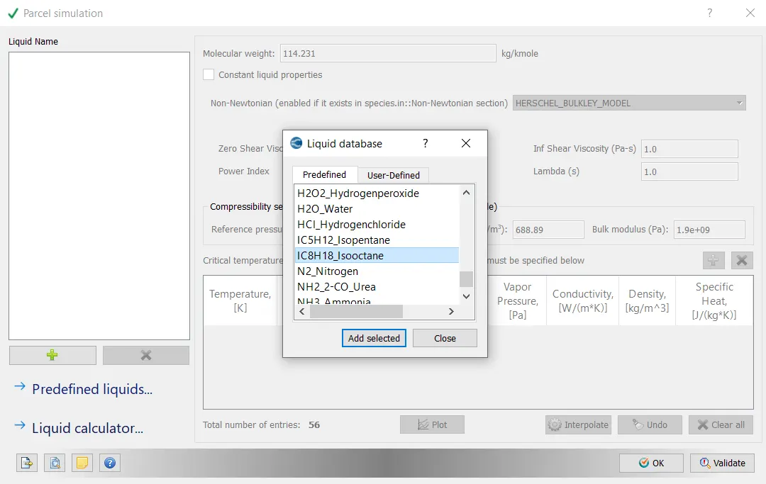
In the Parcel simulation section, from the predefined liquids section select Iso-octane (`IC_8H_18`) and click on
"Add selected". The fuel is selected as Iso-octane because the thermal properties of Iso-octane are similar to that of gasoline.
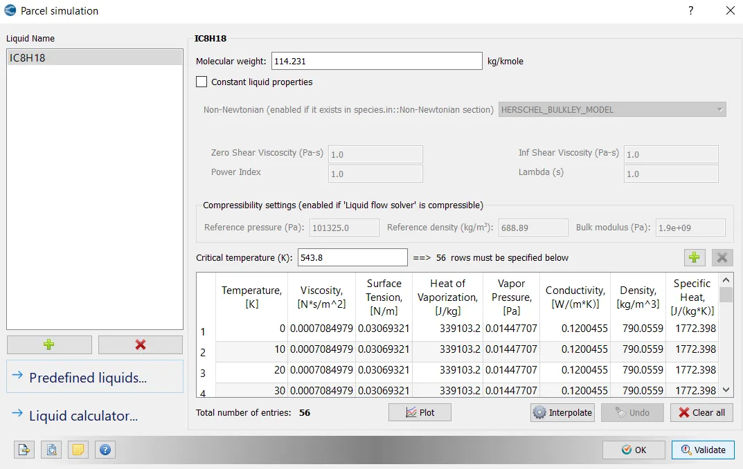
After adding this, it can be seen that the thermal and physical properties of Iso-octane have been obtained as a function of temperature.
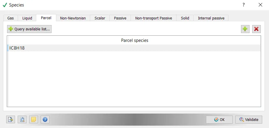
In the species section, under the parcel tab, from the query available list option, Iso-octane (`IC_8H_18`) is added.
Simulation parameters:
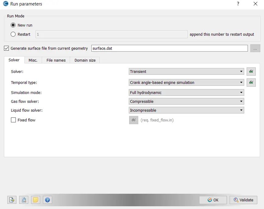
Under the run parameters section the simulation mode is selected as "Full hydrodynamic".
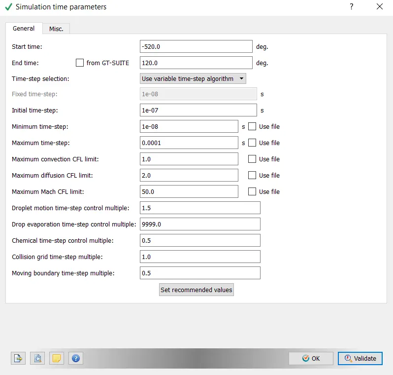
Under the simulation time parameters section, the start time is set as -520.0 degrees and the end time is set as 120 degrees.
Physical Models:
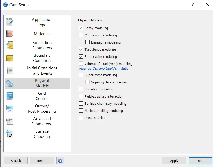
In the physical models, Spray modelling, combustion modelling, Source/sink modelling is checked.
i) Spray modelling:
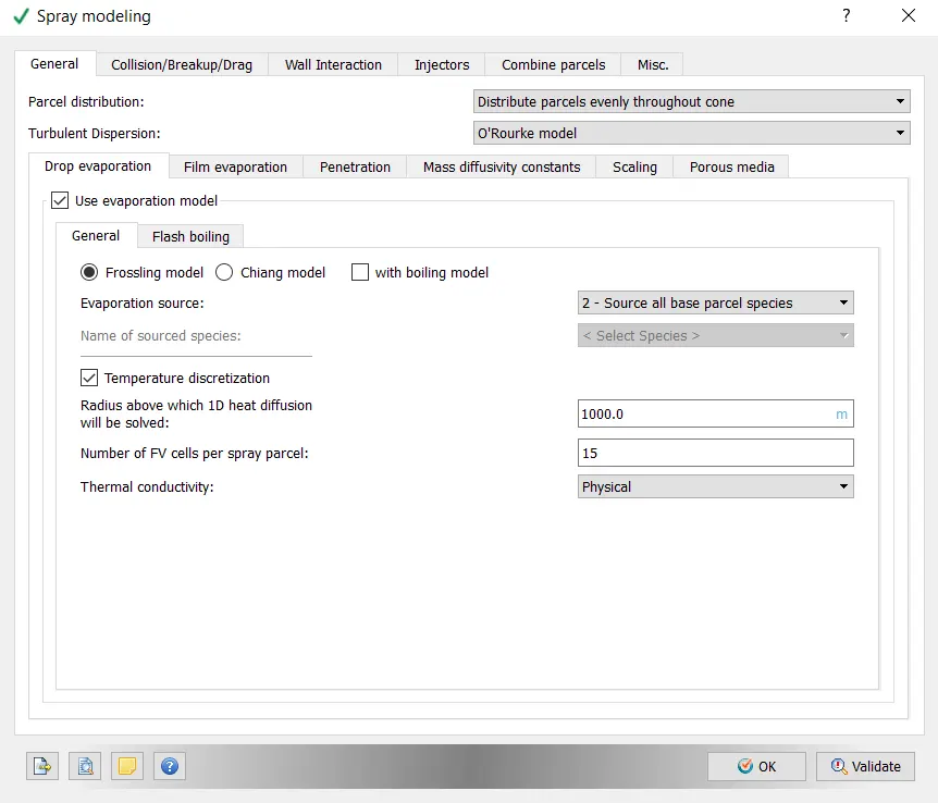
Under the spray modelling section, the general tab is selected and the following settings are done.
Parcel distribution: "Distribute parcels evenly throughout cone" is selected from the drop down box.
Turbulence dispersion: "O'Rourke model" is selected from the drop down box.
Under the Drop evaporation tab,
Evaporation source: "2-Source all base parcel species" is selected from the drop down box.
Temperature discritization is checked.
Radius above which 1D heat equation will be solved is set as 1000.0 m and remaining settings are set as default.
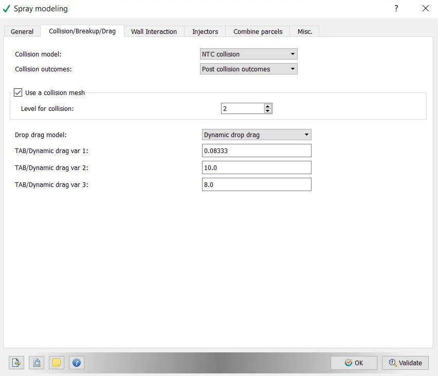
Under the Collision/Breakup/Drag tab, "Use a collision mesh" is checked and the rest of the settings are set as default which can be seen in the image below.
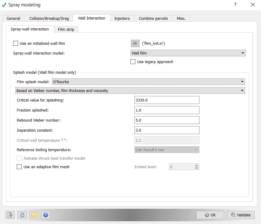
Under the wall interation tab, all the options are set as default which can be seen in the image below.
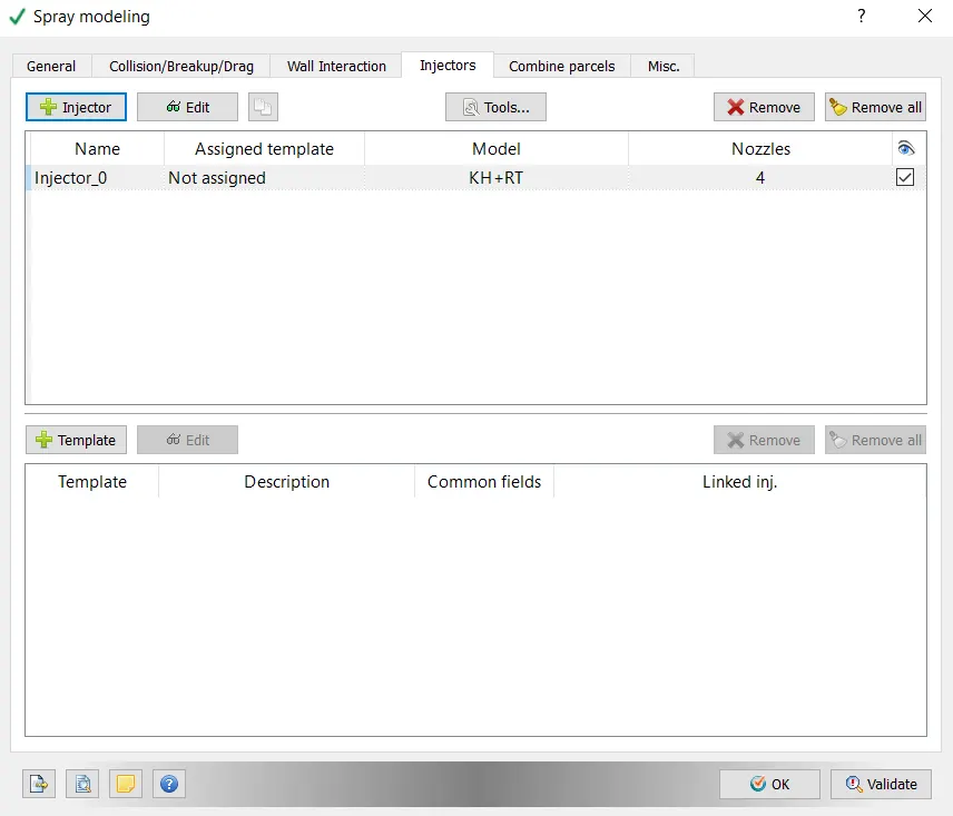
Under the Injectors tab, one injector is added.
The injector is selected and edit option is clicked.
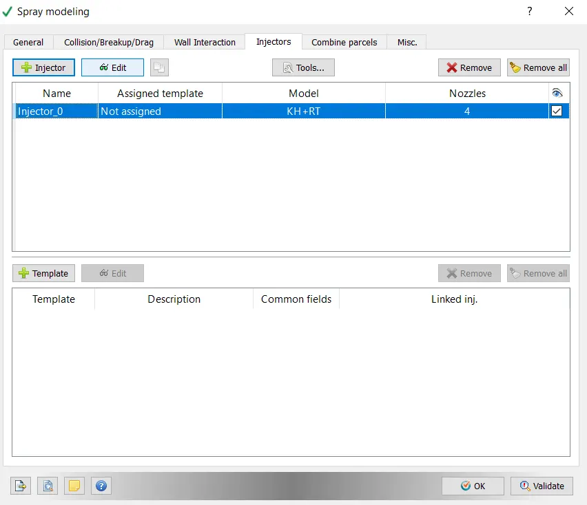
Iso-octane (`IC_8H_18`) is added as the injected parcel species and its mass fraction is set as 1.0.
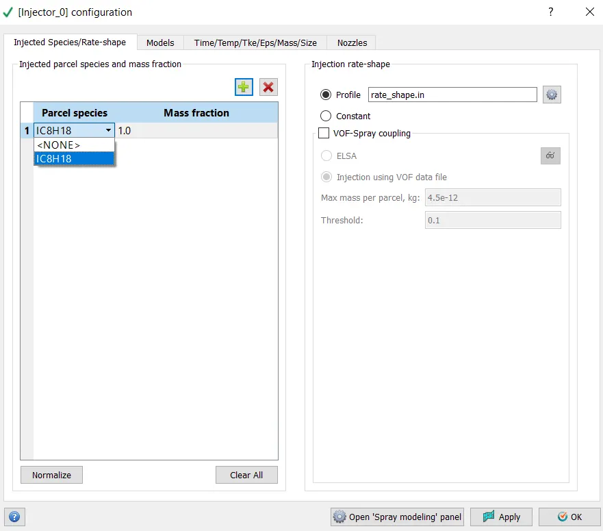
In the injection rate-shape, the profile option is selected and the rate shape file is selected and the profile is set as shown in the image below and the a suitable file name is given with an extension of .in.
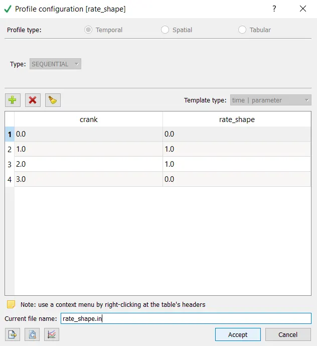
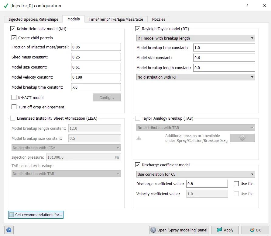
In the models tab, select the Kelvin-Helmholtz model (KH) and Rayleigh-Taylor model (RT) and Discharge co-efficient model. Set the discharge co-efficient value as 0.8.
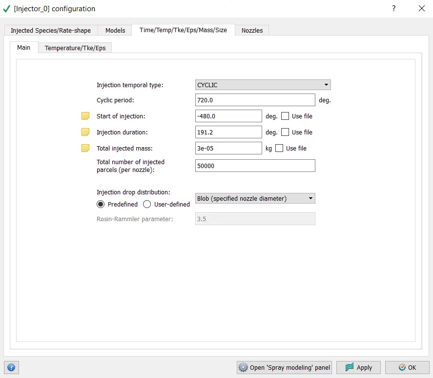
Under the Time/Temperature/TKe/Eps/Mass/Size tab, in the Main section, set the following:
Injection temporal type: "CYCLIC" is selected from the drop down box.
Cyclic period: 720 degrees.
Start of injection: -480.0 degrees
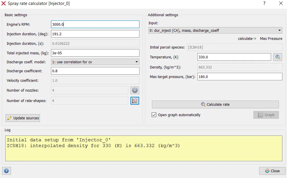
Duration of injection: 191.2 degrees
Total injected mass:
The total injected mass per cycle is calculated as shown below.
Fuel flow rate: `7.5*10^-4` kg/s
R.P.M : 3000
Now, R.P.S will be 50
one revoution is equivalent to 360 degrees.
So, degrees per second will be 50x360= 18000
Time per degree will be `1/18000`= `5.55556*10^-05` `s-deg^-1`
Now, time per 720 degrees is `(5.55556*10^-05 )/720` = 0.04 `s-(720deg)^-1`
Therefore fuel mass per cycle = fuel flow rate x time per 720 degrees ( or 1 cycle of 4 strke IC engine)
= `0.04*7.5*10^-4`
= `3.00*10^-5`
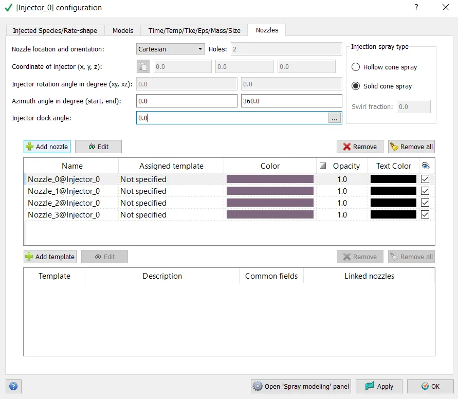
Under the nozzles tab set the following:
Add four nozzles.
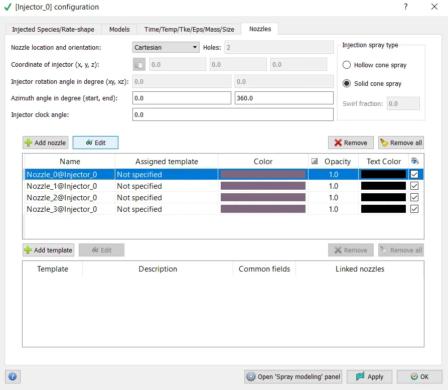
Select the first nozzle and click on edit to edit the first nozzle.
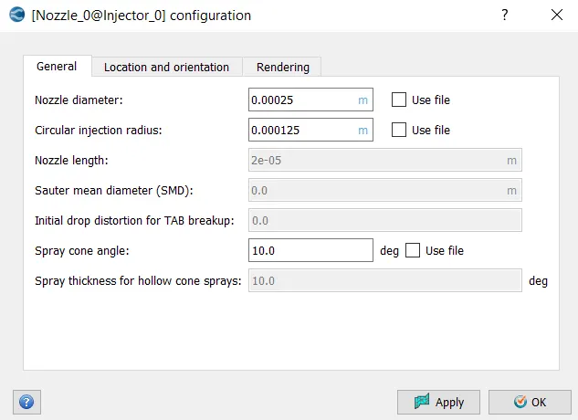
In the general tab, set the following:
Nozzle diameter: 0.00025m
Circular injection radius: 0.000125m
Spray cone angle: 10.0 deg.
In the Location and orientation tab, set the following:
Co-ordinate of nozzle (x,y,z): ( 0.0823357, 0.00100001, 0.07019)
Spray Orientation vector (x,y,z): (-0.732501 0.210489 -0.647408)
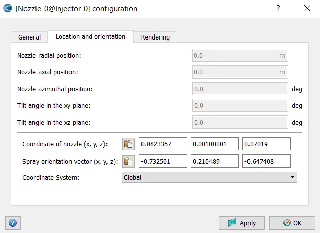
Similarly select the second nozzle and set the following:
In the generals tab,
Nozzle diameter: 0.00025m
Circular injection radius: 0.000125m
Spray cone angle: 10.0 deg.
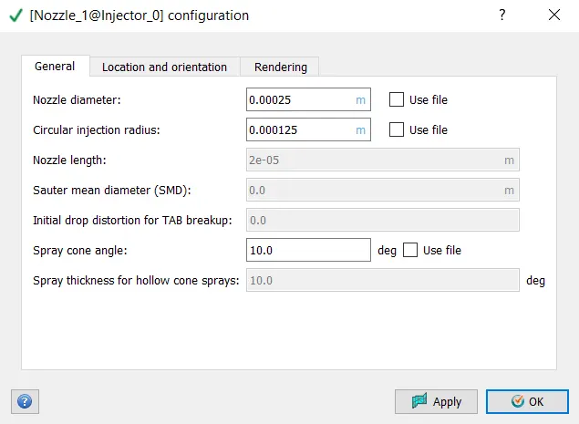
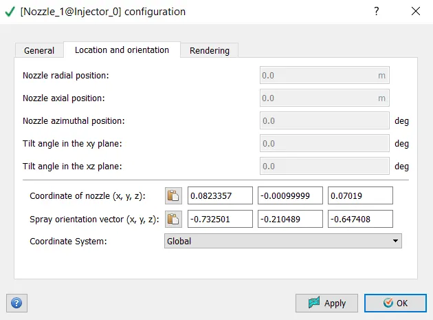
In the Location and orientation tab, set the following:
Co-ordinate of nozzle (x,y,z): ( 0.0823357, -0.00099999, 0.07019)
Spray Orientation vector (x,y,z): (-0.732501 -0.210489 -0.647408)
Similarly select the third nozzle and set the following:
In the generals tab,
Nozzle diameter: 0.00025m
Circular injection radius: 0.000125m
Spray cone angle: 10.0 deg.
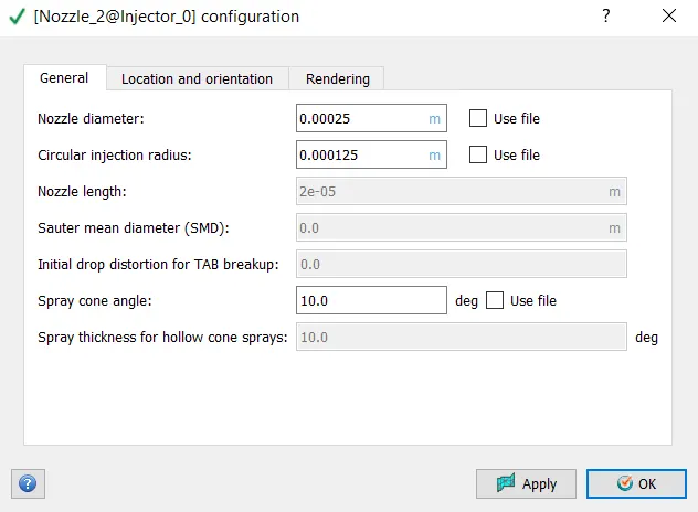
In the Location and orientation tab, set the following:
Co-ordinate of nozzle (x,y,z): ( 0.0823357, -0.0004, 0.07019)
Spray Orientation vector (x,y,z): (-0.5, -0.2, -0.647408)
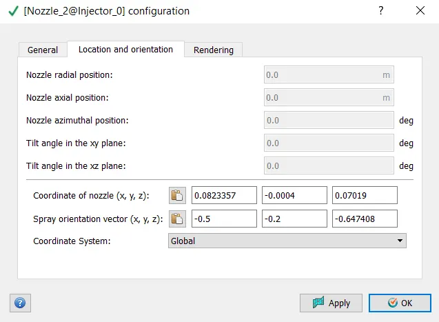
Similarly select the fourth nozzle and set the following:
In the generals tab,
Nozzle diameter: 0.00025m
Circular injection radius: 0.000125m
Spray cone angle: 10.0 deg.
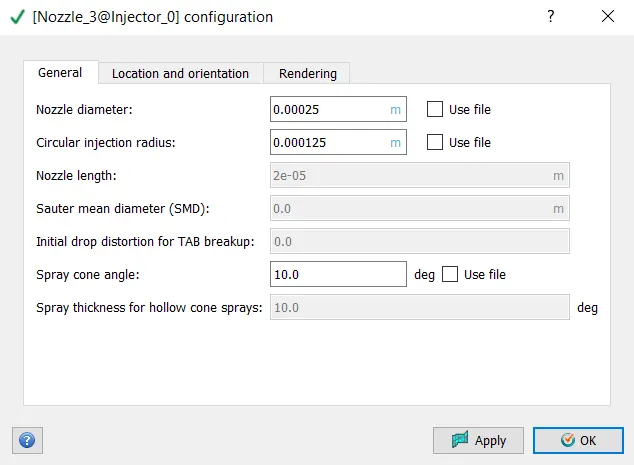
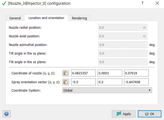
In the Location and orientation tab, set the following:
Co-ordinate of nozzle (x,y,z): ( 0.0823357, 0.0003, 0.07019)
Spray Orientation vector (x,y,z): (-0.5, -0.2, -0.647408)
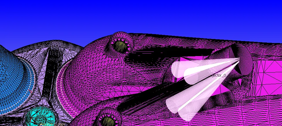
Below image shows the nozzles and injector.
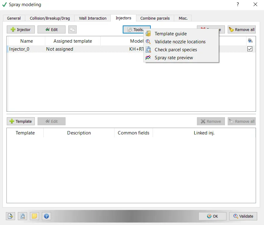
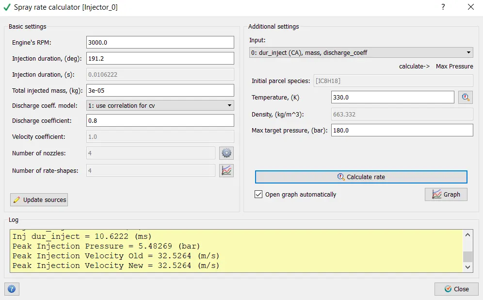
Now, the spray modelling is completed. From the tools in the injector tab the properties of the spray such as pressure, temperature can be previewed. For this the Spray rate preview selected from the tools option.
Check the inputs provided and modify if required. Then click on Calculate rate. After that click on the plots icon.
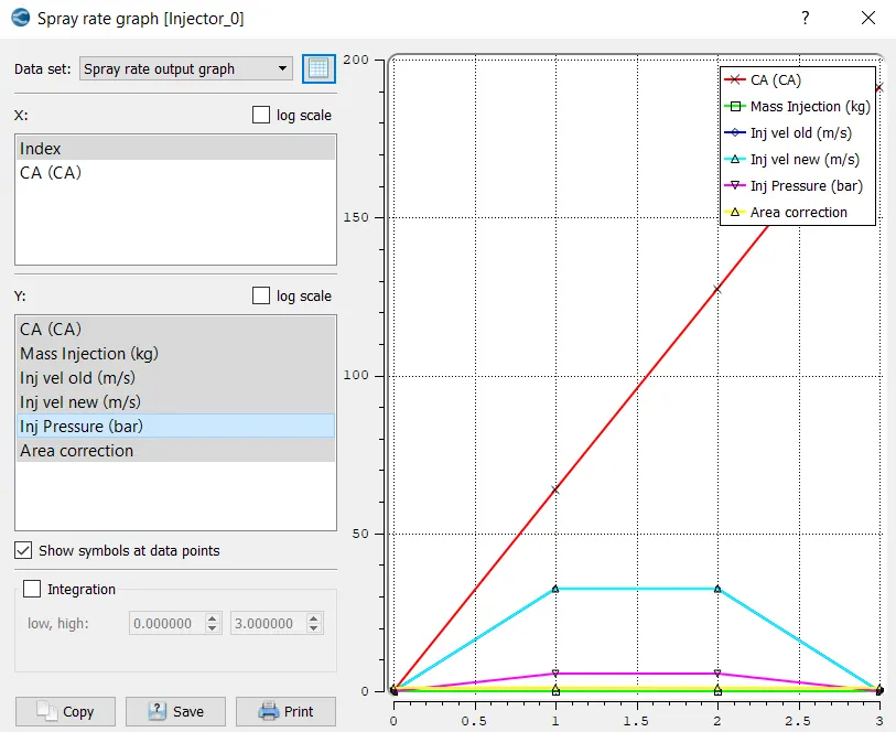
Now, many quantities are plotted as a function of crank angle as it can be seen from the image below. Now, select the injection pressure to see the plot between the injection pressure vs crank angle.
The peak pressure is observed at 5.4869 barfrom the plot which is in the feasibe range for the gasoline engine.
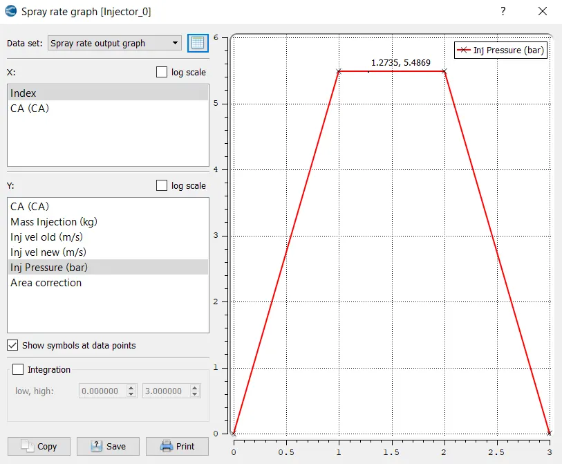
The peak pressure can be verified in the log as 5.48269 bar which matches with the peak pressure in the plot.
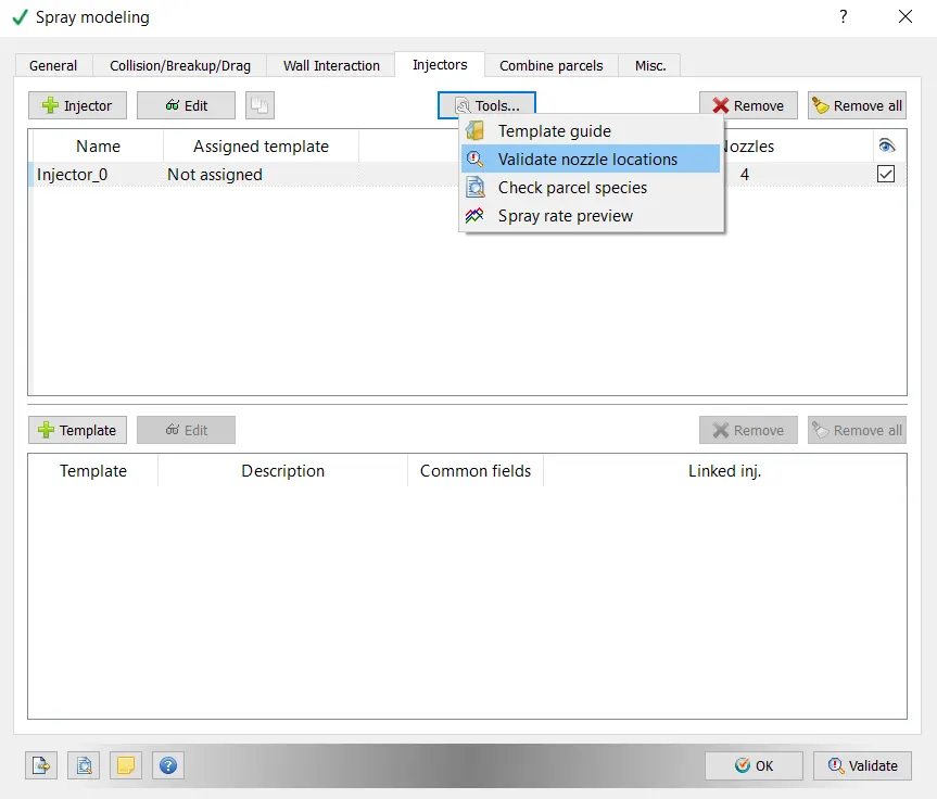
The nozzle locations can also be verified. To do this, Validate nozzle locations option is selected from tools option.
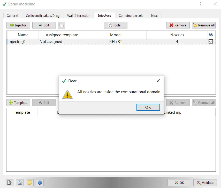
From the below image it can be seen that all the nozzles are inside the computational domain which means that the nozzles are verified.
ii) Combustion modelling:
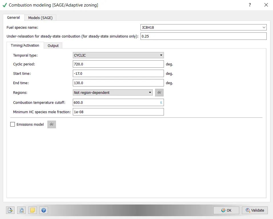
In the combustion modelling section, under the general tab, set the following,
Full species name: `IC_8H_18`
Under relaxation for steady state combustion (for steady state combustions only): 0.25
Under the Time/Activation tab,
Temporal type: CYCLIC is selected from the drop down box.
Cyclic period: 720.0 degrees.
Start time: -17.0 degrees.
End time: 130.0 degrees
Combustion temperature cut-off: 600.0 k
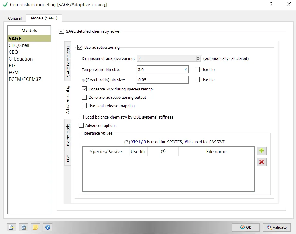
Under the Models,
Check the SAGE detailed chemistry solver.
iii) Source/sink modelling:
Add two sources.
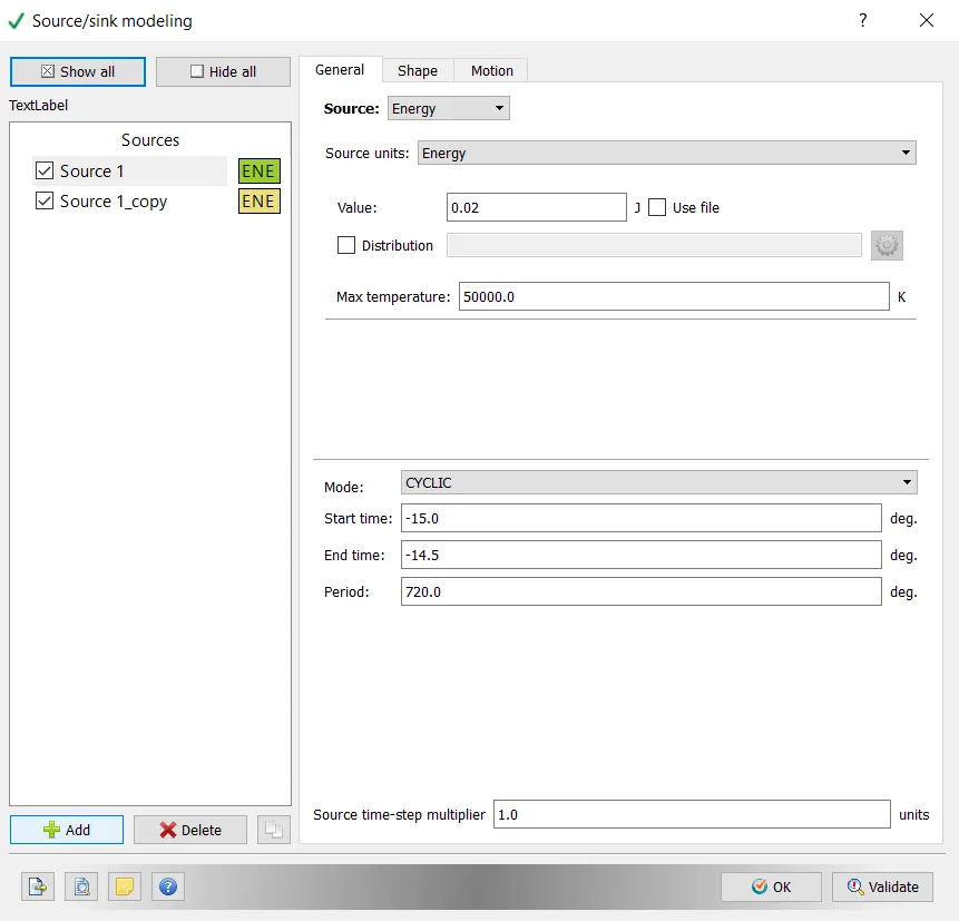
Set the following for source 1:
Under the general tab:
Value of energy: 0.02 joules
Mode: CYCLIC is seected from the drop down list
Start time: -15.5 degrees
End time: -14.5 degrees
Period: 720 degrees
Under the shape tab
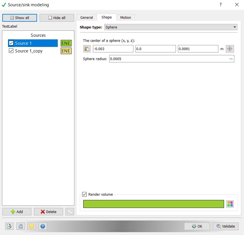
select the shape type: sphere
The center of sphere (x,y,z) = (-0.003, 0.0, 0.0091) m
Sphere radius: 0.0005 m
Set the following for source 2:
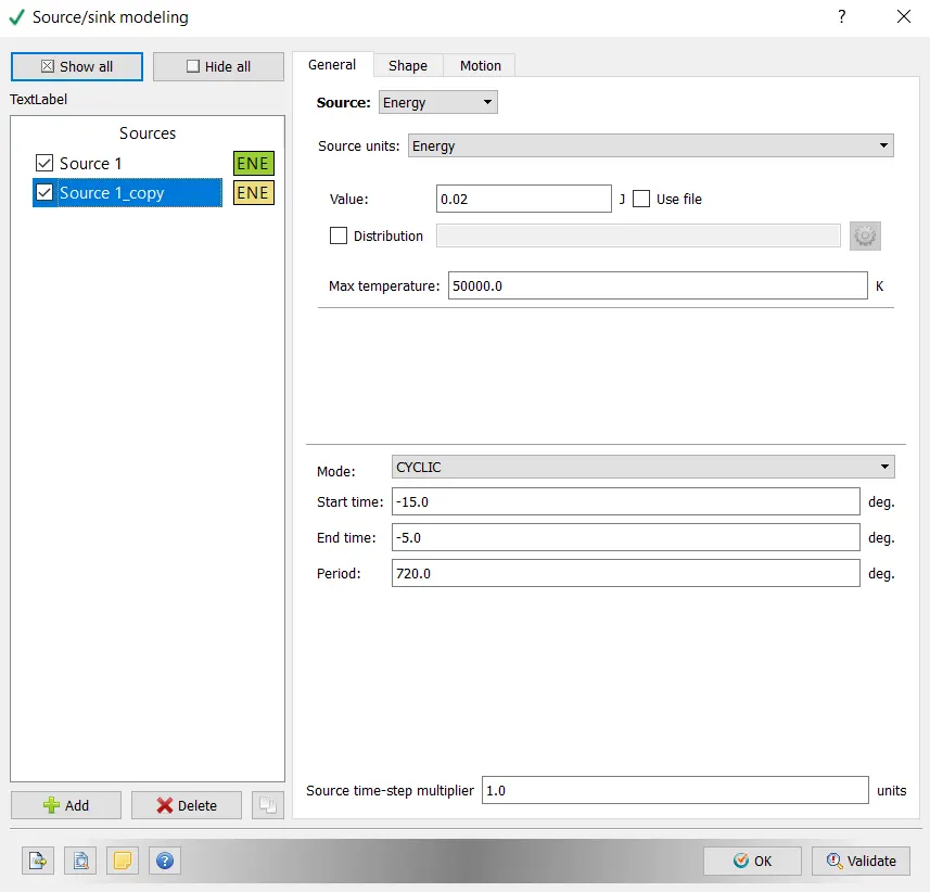
Under the general tab:
Value of energy: 0.02 joules
Mode: CYCLIC is seected from the drop down list
Start time: -15.5 degrees
End time: -5.0 degrees
Period: 720 degrees
Under the shape tab
select the shape type: sphere
The center of sphere (x,y,z) = (-0.003, 0.0, 0.0091) m
Sphere radius: 0.0005 m
It is the same as source 1.
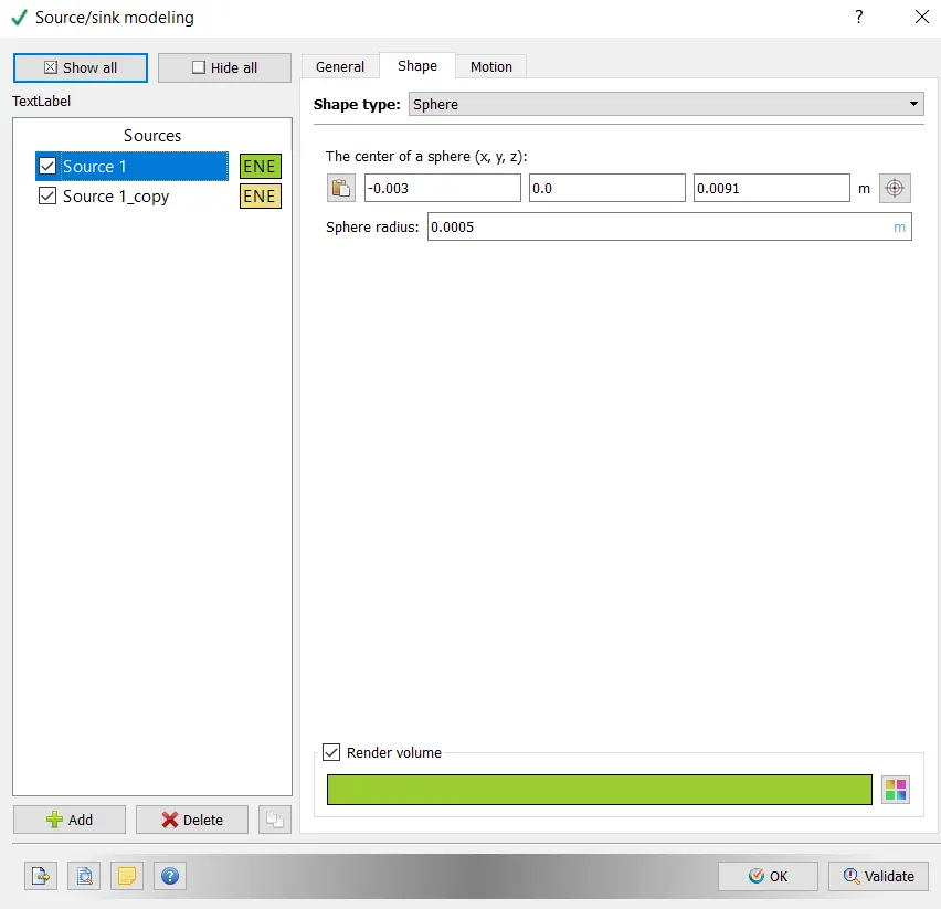
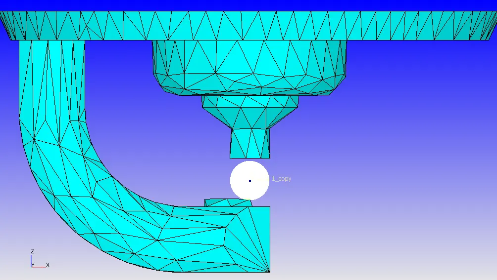
Below image shows the two sources that have been created.
GRID CONTROL:
Check Adaptve mesh refinement.
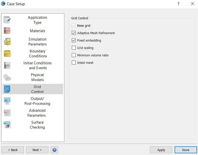
i) In the adaptive mesh refinement section, add one AMR group.
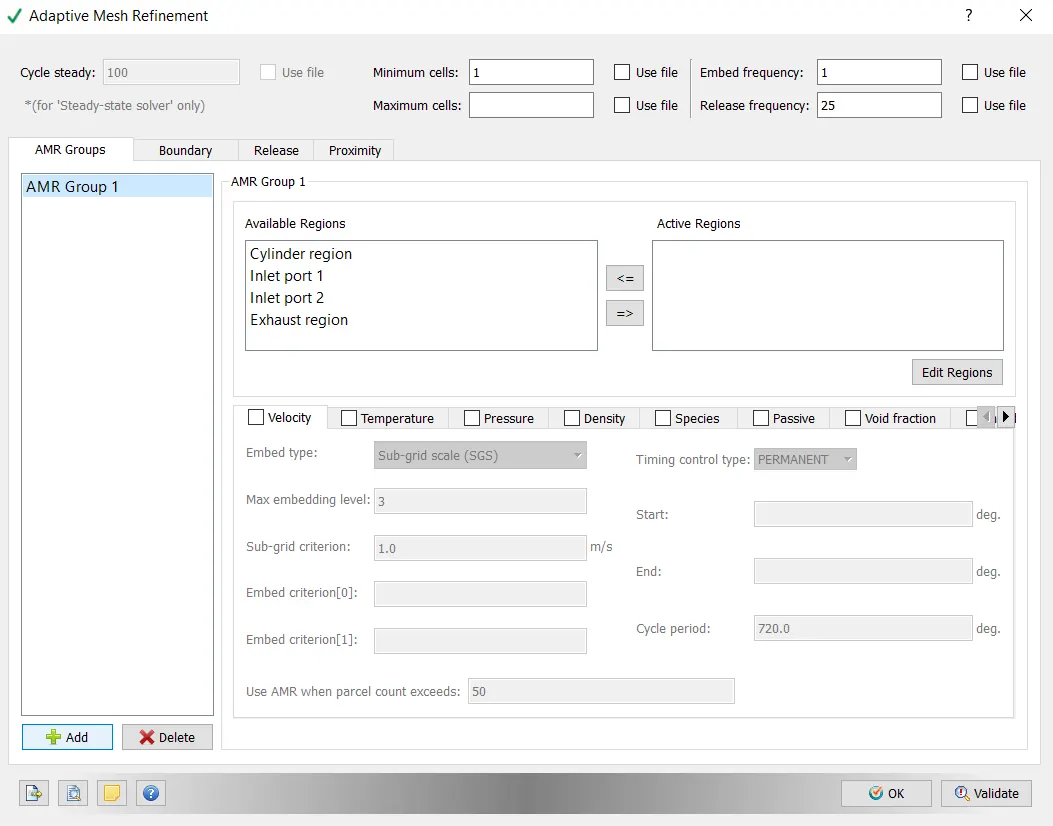
Select all the regions except for Exhaust region in the available region and transfer the selected regions to the active regions.
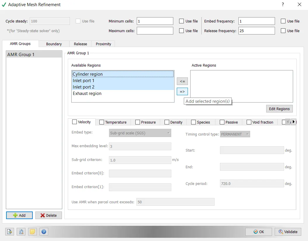
Check velocity and set the following under the velocity tab:
Embed type: Sub-grid Scale (SGS)
Maximum embedding level: 3
Sub-grid criterion: 1.0.
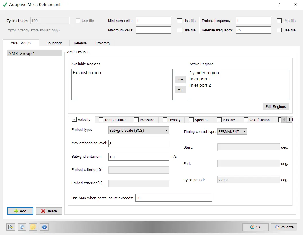
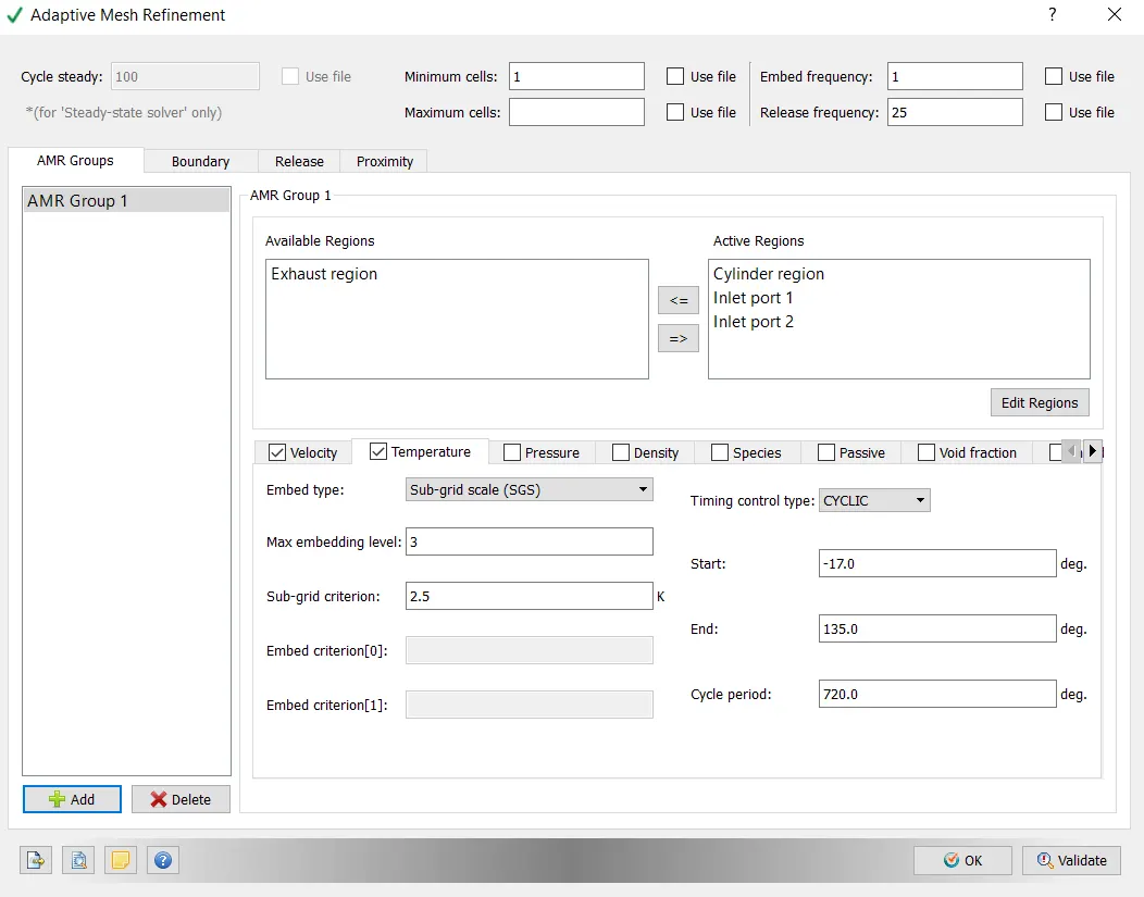
Check temperature and set the following under the temperature tab:
Embed type: Sub-grid Scale (SGS)
Maximum embedding level: 3
Sub-grid criterion: 1.0.
Timing control type: CYCLIC is selected from the drop down list.
Start: -17.0
End: 135.0
Cycle period: 720.0
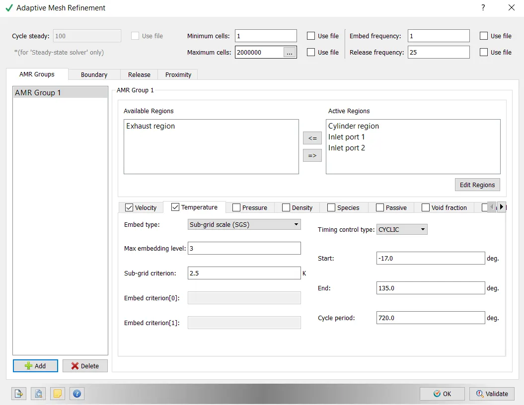
Maximum cells are set as 2000000
ii) In the Fixed embedding section add three more embedding namely, Spherical embedding, Larger sphere, Injector embedding.
For Spherical embedding set following:
Entity: SPHERE
Mode: CYCLIC
Period (cyc. mode): 720.0 degrees
Scale: 5
Start: -16.0
End time: 7.0 degrees
The centre of a sphere: (-0.003, 0.0, 0.0091) m
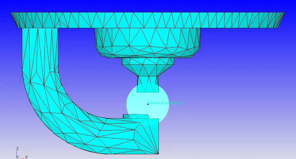
radius of sphere: 0.001m.
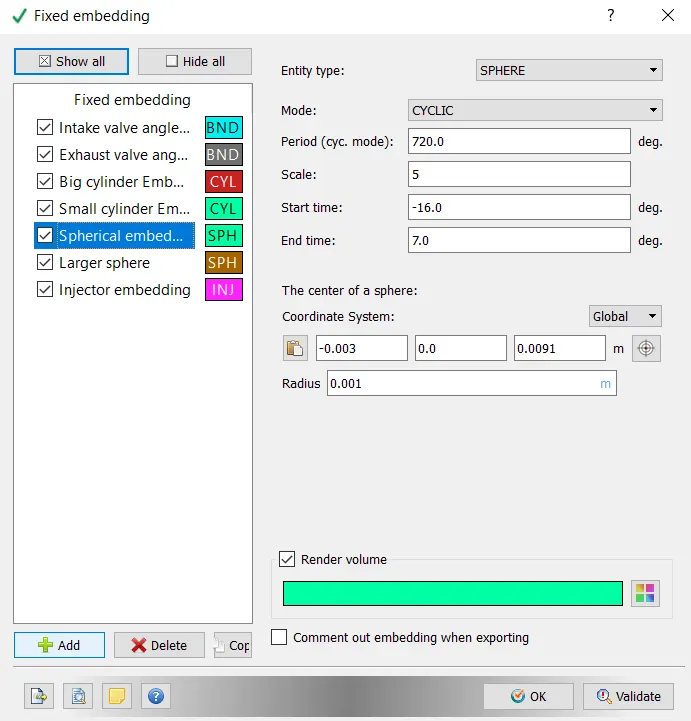
Below is an image showing the spherical embedding.
For Larger sphere embedding set folowing:
Entity: SPHERE
Mode: CYCLIC
Period (cyc. mode): 720.0 degrees
Scale: 3
Start: -16.0
End time: 7.0 degrees
The centre of a sphere: (-0.003, 0.0, 0.0091) m
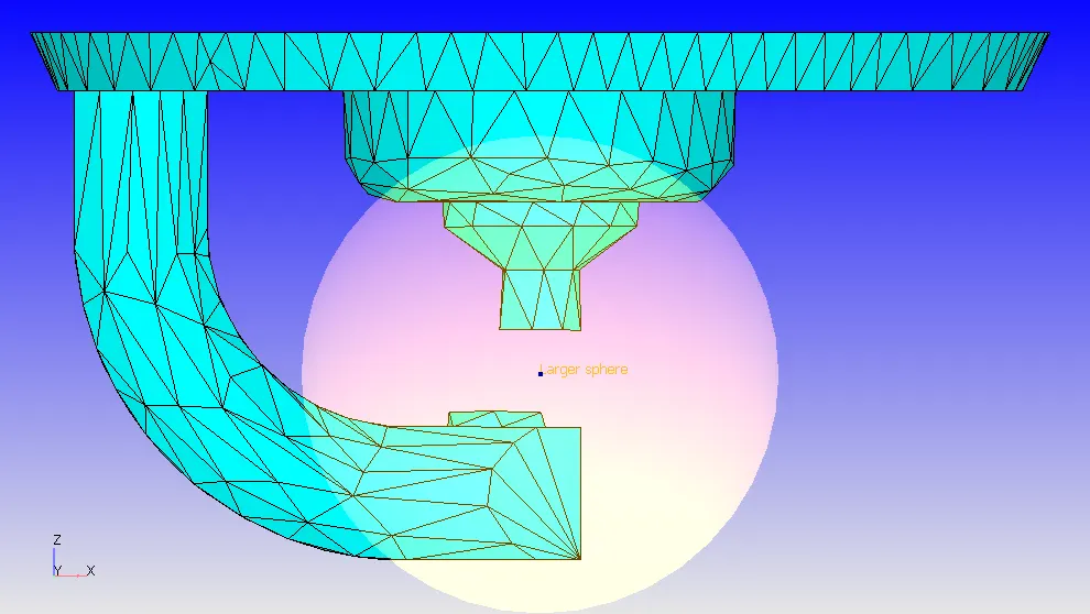
radius of sphere: 0.003m.
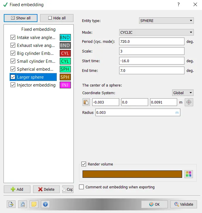
Below is an image showing larger sphere embedding.
For Injector embedding set following:
Entity: INJECTOR
Mode: CYCLIC
Period (cyc. mode): 720.0 degrees
Scale: 4
Start: -482.0 degrees
End time: -286.0 degrees
Injector ID: Injector_0 is selected from the drop down list.
Radius 1: 0.002 m
Radius 2: 0.004 m
Length: 0.02 m
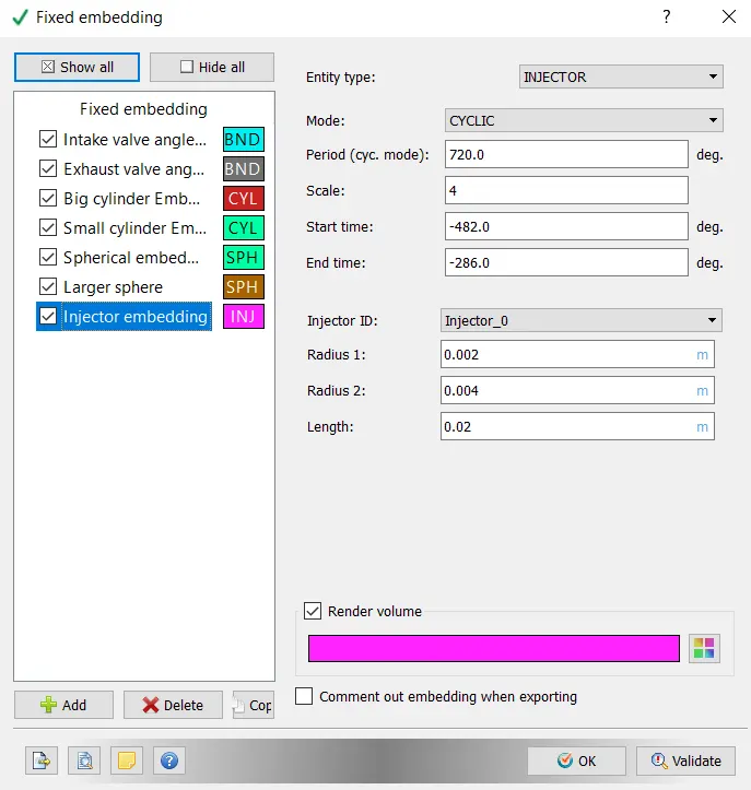
Below is an image showing injector embedding

Mesh refinement due to fixed embedding and Adaptive mesh refinement:
Fixed embedding: Fixed embedding is a type of grid control technique used in converge. This technique refines the mesh size at a particular selected cells of a boundary or a region or a particular part of the geometry for which the simulation is done. This refinement can last upto a specific time during the simulation or it can also be present throughout the simulation. The amount of refinement can be regulated by using the Scale of embedding.
If embedding scale is 'n' then the refined cell size = `("base grid")/2^n`
So, for the spherical embedding the scale is set to 5and the base grid size is 0.004 m.
Therefore, the refined cell size = `0.004/2^5` = 0.000125m.
The duration for the above embedding is from -16 degrees to 7 degrees.
For the large sphere, the embedding scale is 3, therefore the refined cell size = `0.004/2^3`= 0.0005m
The duration for the above embedding is from -16 degrees to 7 degrees.
For the Injector embedding, the embedding scale is 4, therefore the refined cell size = `0.004/2^4`=0.00025m
The duration for the above embeding is from -482 degrees to -286 degrees.
Adaptive mesh refinement: Adaptive mesh refinement is a type of grid control technique used in converge. This technique uses a criterion called sub-grid scale to refine the cells. If a quantity is fluctuating from large values to very small values and the range of fluctuation is high, then it will be very difficult to capture exactly all the data during the simulation as the change in the quantity under study is high. In this case, adaptive mesh refinement can be used. If the difference in the quantity between the two adjacent cells is more than a specified value called sub-grid scale criterion, then these cells get refined. So, unlike fixed embedding whose duration of occurance is fixed by the user, the adaptive mesh refinement adapts itself to when and where the sub-grid scale criterion is met. Thus, this technique is highly useful when the time and place of refinement of the cells is complex and does not follow a simple pattern.
For example, the quantity which varies a lot during the simulation is considered as temperature.
If in between any two sub-grids there exists a temperature difference that exceeds the value of sub grid scale temperature difference, the Adaptive mesh refinnement applies to those sub-grid cells and the cells get refined into more finer cells. This uneven, dynamic distribution of cells which changes according to the detailness of a particular quantity under study and at the particular time of requirement during the simulation is called Adaptive mesh refinement.
In Adaptive mesh refinement, the finest cells can be calculated as:
Finest cells = `("Base Grid size")/(2^("maximum embedding level"))`
In this PFI engine, in the velocity AMR,
The sub-grid scale criterion is 1.0 m/s.
So, if the veocity difference between the two adjacent cells is more than 1.0 m/s, those cells get refined as follows:
Refined cells = `("Base Grid size")/(2^("embedding level"))` = `0.004/2^1` = 0.002 m.
If those adjacent cells' velocity difference is still greater than 1.0 m/s then they get refined by one more embed level, and the refined cells have a size of 0.001m.
And if the velocity difference is still greater than 1.0 m/s, the cells get refined again by one embed level which gives the refined cells with a size of 0.0005m.
As the maximum embedding level is set as 3 for velocity AMR, the smallest cell size that can be obtained is 0.0005m.
Similarly, for temperature AMR,
The sub-grid scale criterion is 2.5k.
So, if the temperature difference between the two adjacent cells is more than 2.5k, those cells get refined as follows:
Refined cells = `("Base Grid size")/(2^("embedding level"))` = `0.004/2^1` = 0.002 m.
If those adjacent cells' temperature difference is still greater than 1.0 m/s then they get refined by one more embed level, and the refined cells have a size of 0.001m.
And if the temperature difference is still greater than 1.0 m/s, the cells get refined again by one embed scale which gives the refined cells with a size of 0.0005m.
As the maximum embedding level is set as 3 for temperature AMR, the smallest cell size that can be obtained is 0.0005m.
Valve profiles:
The below file contains the exhaust valve profile at different crank angles during the simulation.
The below file contains the intake valve profile at different crank angles during the simulation.
Importance of Regions and Events:
Regions in converge are a group of boundaries. These can be used to provide different initial conditions to different parts of a geometry. Events in converge studio, are used to connect or disconnect two regions. Events can be very helpful in simulating some cases where we it is requried to break some part of the geometry at a particular time such as breaking a diaphragm in a shock tube. Also, in some cases it may be required to connect the valve in the inlet port of a PFI engine at a particular time and disconnect them when not required.
Importance and need of ring triangles:
The ring triangles are made at the interface of the valve top and the ports (intake and exhaust). In the boundary flagging, the ring triangles are flagged to ports (Inlet and exhaust) as shown in the below image. This is done to avoid the distortion in shape of the portion of exhaust port near the ring triangles when it is required to translate the valve before setting up the case.
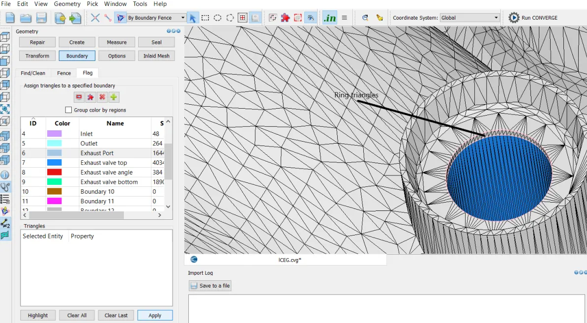
If the ring triangle is not present and if the valve position while surface preparation is found to be not correct, then when the valve is tried to translate, the portion of the port near the valve top gets pulled toawrds the direction of translation of the valve thereby distorting the shape of the port at the interface with the valve top. If the ring triangles are present then instead of the exhaust port, the ring triangles whose curvature is same as that of the valve top, get extended hence the distortion of the port is avoided.
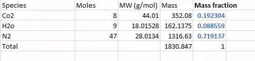
Calculation of mass fraction of species which are present in combustion chamber and exhaust:
The combustion reaction is assumed to be stoichiometric and the balanced reaction is shown below.
`C_8H_18 + 12.5.(O_2 + 3.76N_2) -> 8CO_2 + 9H_2O + 12.5*3.76N_2`
The mass fraction calculations are shown below:
RESULTS AND DISCUSSION:
1) Plot of volume of air and other gases in the cylinder vs crank angles:
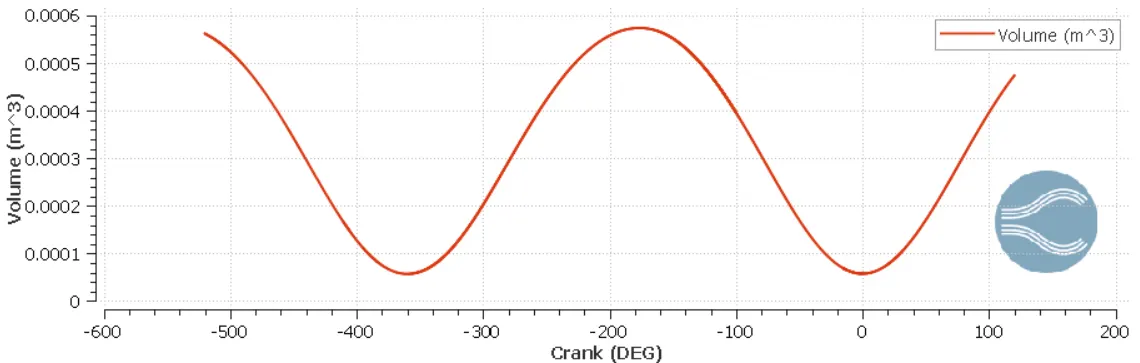
From the above plot it can be observed that the air volume iinside the cylinder is maximum at the beginning at -520 degrees crank angle, which means that the piston is at the bottom dead centre. As the piston moves towards the top dead centre, the air compresses and as a result the air volume decreases. It reaches its minimum value at the top dead centre. At this point the compression stroke is complete and ignition takes place. Due to energy released after combustion, the piston is pushed towards the bottom dead centre and hence the volume of the air and other combustion gases increases. This is the power stroke. After this, the combustion flue gases are sent outside the cylinder through the exhaust, during which the piston moves from bottom dead centre to top dead centre, decreasing the air volume again. After this the air from the inlet valve is allowed in to the cylinder as the piston moves from top dead centre to bottom dead centre.
Compression ratio of this engine:
Compression ratio of an engine is given by the ratio of maximum air volume inside the cylinder to the minimum air volume inside the cylinder which is `V_max/V_min`.
From the above plot between air volume inside the cylinder vs crank angles, the maximum and minimum volumes of the air can be obtained.
`V_max`= `5.742*10^-4``m^3`
`V_min`=`5.702*10^-5``m^3`
Therefore compression ratio = `V_max/V_min` = `(5.742*10^-4)/(5.702*10^-5)` = 10.07
2) Plot of Pressure of air and other gases inside the cylinder vs crank angle:
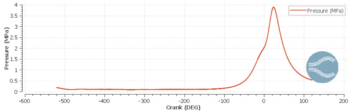
From the above plot it can be observed that the pressure of air inside the cylinder increases gradually and then as the fuel injection starts at the end of compression stroke, the pressure inside the cylinder increases rapidly and the fuel molecules reaches their ignition temperature and the combustion starts. This is reflected in the graph as the slope of the above curve suddenly increases and thus the pressure reacches its maximum value. After this, the pressure starts to decrease as the piston completes its power stroke.
3) Plot of Mean temperatuure inside the cylinder vs crank angles:
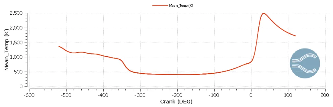
From the above plot it can be observed that the mean temperature inside the cylinder reaches its maximum value during the combustion of the fuel. It can also be observed that the pressure inside the cylinder is also at its maximum right around the same crank angle.
If someone does a thermal analysis using a software like ANSYS, then the gas side boundary conditions. There this profile can be given as an input.
4) Plot of Mass inside the cylinder vs the crank angle:
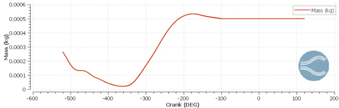
From the above plot the mass inside the cylinder can be known at every crank angle during the entire cycle of engine. The mass in side the cylinder after the exhaust stroke is the mass which is trapped inside the cylinder. This is a very important quantity as it indicates wheteher there is any unburnt fuel left inside the cylinder after the cycle ends. For an efficient engine, the trap mass should be minimum.
5) Plot for Heat release rate vs crank angle:
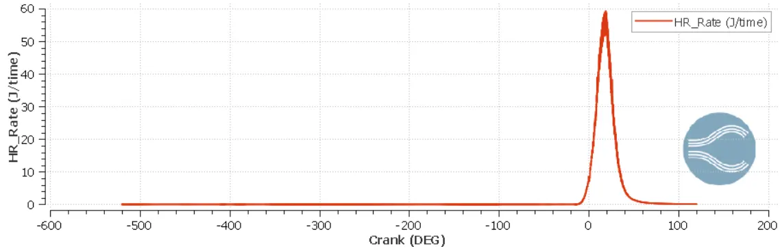
From the above plot, the heat release rate per degree of crank angle is constant until combustion occurs and as the combustion process releases heat energy, the rate of heat released during that period increases rapidly. Then, afterwards the heat release rate decreases as the comustion ends.
6) Plot for Integrated heat release rate vs crank angle:
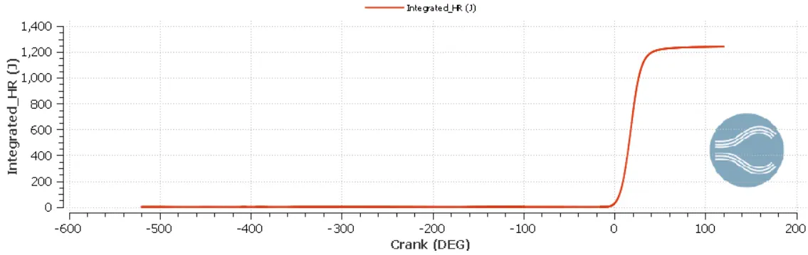
The heat release rate is integrated and the quantity obtained is called integrated heat release. The value at the end indicates the amount of energy released from combustion alone. By using this, the combustion efficiency of the engine can be calculated. By knowing the combustion efficiency, the quality of an engine in terms of the percentage of fuel used can be judged.From the above plot, the value of the heat released due to combustion= 1241.1626 J.
Combustion efficiency of the engine:
The value of the heat released due to combustion= 1241.1626 J.
Net calorific value of gasoline= 43.4 MJ/kg
Mass of gasoline injected = `3.00*10^-5 kg`
The energy contet of gasoline = Net calorific value of gasoline x Mass of gasoline injected
= `43.4*10^6*3.00*10^-5`
= 1302 J.
Combustion efficiency of the engine = `[("heat released due to combustion")/("the energy content of gasoline")]*100`
= `1241.1626/1302*100`
= `95.33 %`
7) Plot of liquid spray drops inside ethe cylinder vs crank angle:
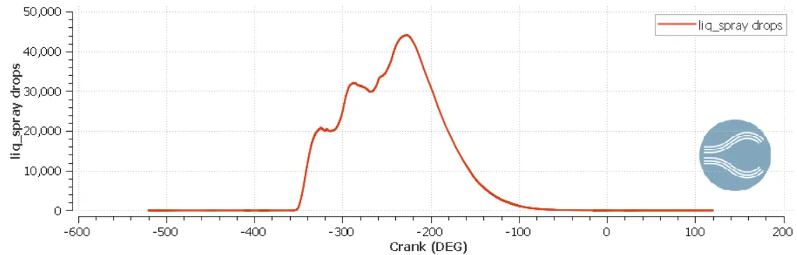
From the above plot it can be observed that the liquid spray drops are zero until the injection of the fuel spray inside the cylinder from the inlet port through the inlet valve. Just after the start of injection, the liquid spray drops increases suddenly and then it decreases for someime which is due to evaporation of some of the drops, Then againn it increases and follows the simlar pattern as the liquid spray drops increases. Then after the injection is complete the liquid spray drops vapourises and after the combustion is complete the liquid spray drops are converted into gasesos flue gases and eventually becomes zero.
8) Plot of iso-octane inside the cylinder vs crank angles:
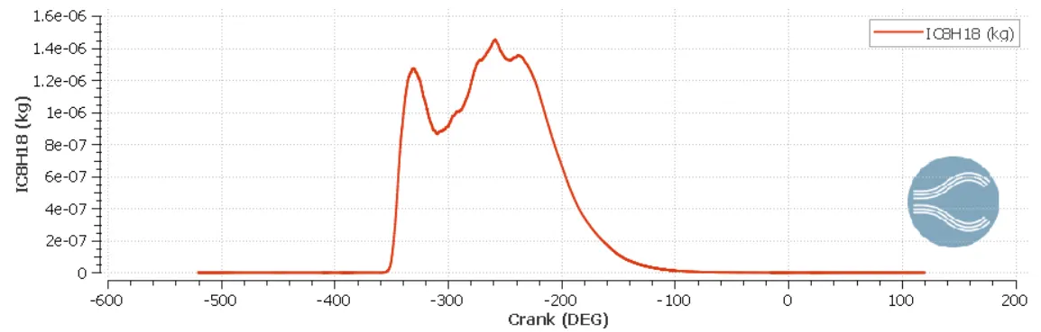
From the above plot it can be observed that the mass of iso-octane is zero inside the cylinder until the fuel is injected. Just after the fuel is injected, the mass of iso-octane increases rapidly and then decreases due to evaporation and vaporisation. Then, after the combustion takes place, the mass of iso-octane is zero which means that iso-octane has been completely burnt.
9) Plot of Mass of combustion products vs crank angles:
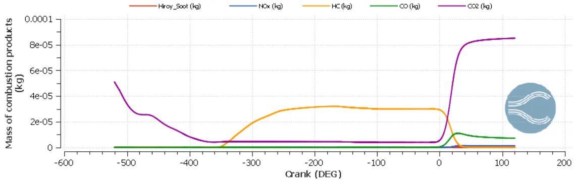
i) Hiroy_soot: It is the amount of soot emitted which is obtained by using the hiroyasu model. It can be observed that the plot is in orange colour. The amount of soot obtained is about 2.53x 10^-8 kg.
ii) `NO_x`: The oxides of nitrogen emitted are about 1.28x 10^-6 kg. The plot is shown in blue colour.
iii) HC: The amount of HC produced is 1.44x 10^-8 kg. The plot is shown in yellow
iv) CO: Carbon monoxide amount produced is 7.11x 10^-6 kg. The plot is shown in green colour.
v) `CO_2`: Carbon dioxie amount produced is 8.51x 10^-5 kg. The plot is shown in violet colour.
The above emissions must be minimized for a better performance and environment friendly engine.
10) Plot for Pressure inside the cylinder vs volume inside the cylnder:
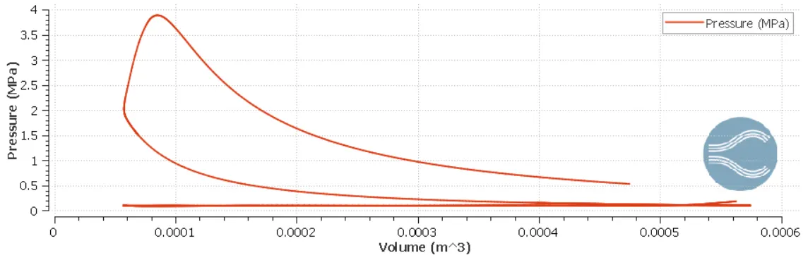
The above plot between the pressure and volume of the cylinder can be used to calculate the amount of work done by the engine throughout the cycle. Converge also provides a tool for calculating the performance parameters of the engine based upon the inputs given to it. Ths is called engine performance calculator.
Work done and many other important perfrmance parameters obtained from the engine performance calculator are as follows:
Work done by the engine: 468.65 N-m
Indicated mean effective pressure (IMEP): 0.8964 MPa
Peak firing pressure: 3.888 MPa
Heat release rate peak: 59.356 J
Caculation of power of engine:
RPM of engine: 3000
Number of revolutions in 1 cycle= 2
Cycles per minute= 1500
Cycles per second= `1500/60`= 25
Work done by the engine per cycle= 468.65 J
Therefore Power of the engine= (work done by the engine per cycle) x (cycles per second)
= 468.65 x 25
= `11.716`Kw
If the frictional losses are neglected then, Brake power = Indicated power.
Calculation of Torque of engine:
Power, P= `(2*pi*n*T)/60`
Therefore, Torque, T= `30*P/(pi*n)`
= `(30*11.716*10^3)/(pi.3000)``N-m`
= 37.294 `N-m`
Significance of Ca10, Ca50 and Ca90:
Ca10 indicates the crank angle at which 10% of combustion has been completed.
Ca50 indicates the crank angle at which 50% of combustion has been completed.
Ca90 indicates the crank angle at which 90% of combustion has been completed.
Need of a wall heat transfer model:
Wall heat transfer is required because the wall temperature cannot be predicted using CFD simulation. As a Computational Fluid Dynamics computes the temperatures for the gas phase, also always the boundary conditions are to be provided in order to run the simulation. Hence a wall heat transfer model is required.
Animations:
Below is the link for an animation showing the temperature of parcels during the simulation.
https://www.youtube.com/watch?v=8cMVssZRcdw
Conclusion:
1) Full hydrodynamic case setup for PFI engine is successfully completed.
2) The compression ratio of this engine is calculated as 10.07 which is typical for an SI engine.
3) The combustion efficiency is obtained as 95.33% which means that 95.33% of the energy content of gasoline is released as heat after combustion.
4) The power of the engine is calculated as 11.716 kw.
5) Torque of this engine is calculated as 37.294 N-m.