Project 1 : Flow over Ahmed Body

Aim:

• To simulate the flow over Ahmed body in such a way that the floor of the wind tunnel must be divided into two sections slip and no-slip condition and find Drag and Lift Coefficient.
• To simulate the flow at two different slant angle that is 25° and 35° and in addition to that apply two turbulence modelling condition for each slant angle ie k-Omega and K-Epsilon
• Validate your velocity profile along the Ahmed body at different points with the experimental data provided.

Theory:

The Ahmed body is a generic car body (a simplified vehicle model). The airflow around the Ahmed body captures the essential flow features around an automobile and was first defined and characterized in the experimental work of SR Ahmed in his research Some salient features of time average ground vehicle wake. Although it has a very simple shape, the Ahmed body allows us to capture characteristic features that are relevant to bodies in the automobile industry.

The simple geometrical shape has a length of 1.044 meters, the height of 0.288 meters, and a width of 0.389 meters. It also has 0.5-meter cylindrical legs attached to the bottom of the body and the rear surface has a slant that falls off which in this challenge have is 35 and 25 degree

Modelling

3d modelling is made by taking the above dimensions and also the width of the extrusion

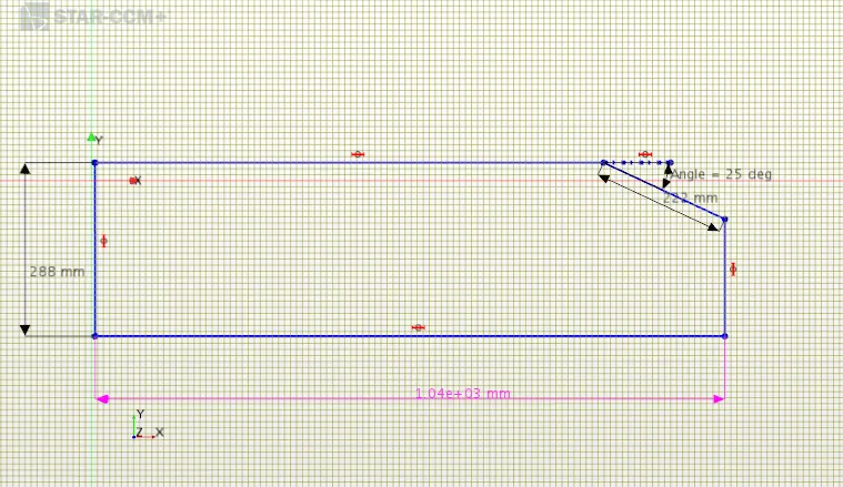
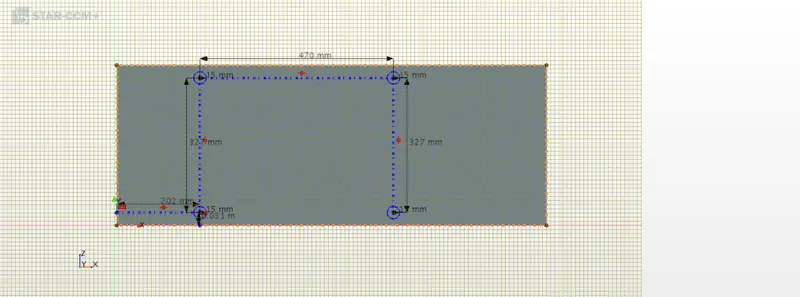
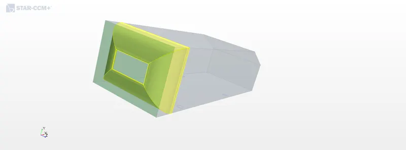
After Modelling of Ahmed body, a wind tunnel is created with a section of floor

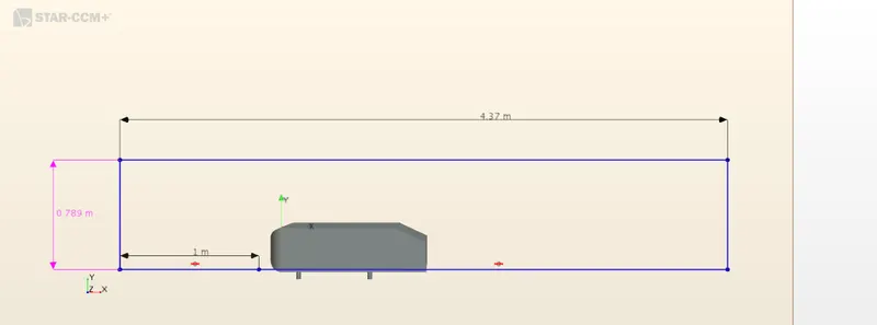
The Two models created are combined to form as one unit. That one combined model is then assigned parts to region Here two things are enabled.

• Create a boundary for each part surface.
• Create a Region fo Region for each part.

The models are labelled by assigning the names

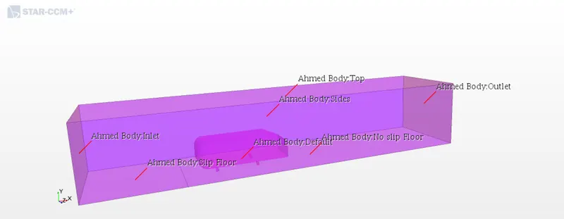
In Regions, boundary types are assigned to each part

Inlet: Inlet Velocity

Outlet: Pressure Outlet

Top, Ahmed Body, Both Floors: Walls

Sides: As Symmetrical Plane

MESHING

The following Meshers are selected

• Surface Remesher.
• Automated Surface Repair.
• Trimmed Cell Mesher.
• Prism Layer Mesher.

Change in the controls

Base Size:0.08m

Maximum cell size:1000%

Y+ is a dimensional quantity through which we can get the first cell height

Here y+ 50 is assumed as wall-functions are used to resolve the near-wall region

The Thickness that came out through y+ of 50 is given below

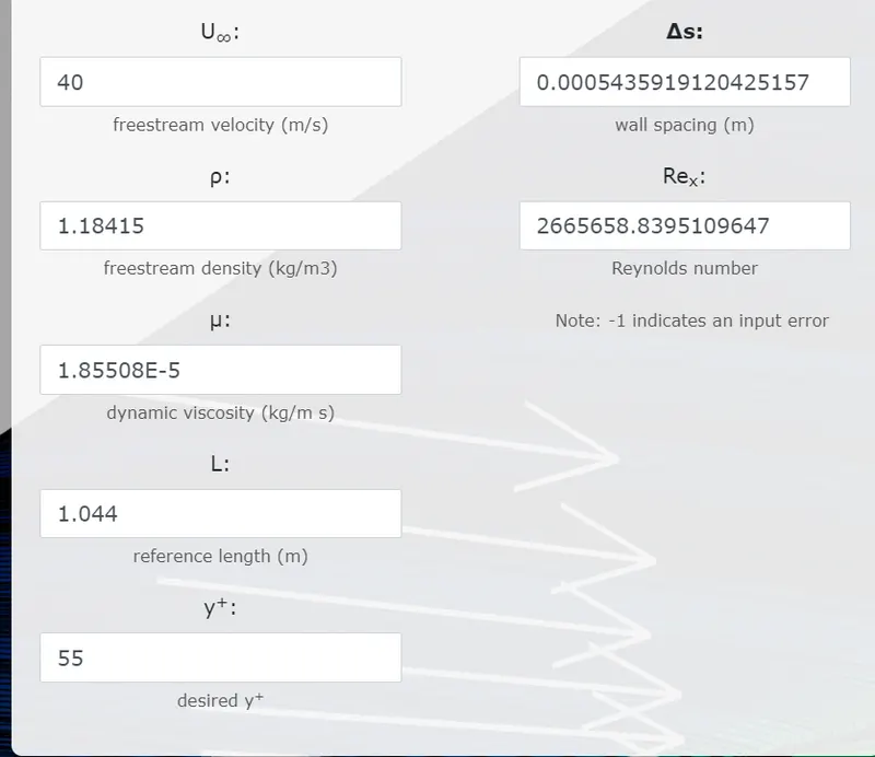
Prism Layer Total Thickness: 0.5mm

Total Number of Prism Layer: 12

Custom Controls -

Surface Control 1

Part : Top,Sides,Inlet,Outlet

Target and Minimum size: 1300% of the base size.

Surface Control 1

Part: Slip and No-slip Floor

Base size :20

Target and Minimum size: 1000% of the base size.

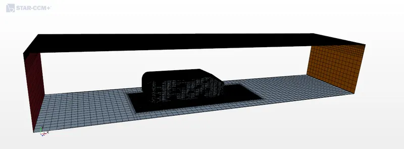
To Capture capture physics more a block is made around Ahmed Body and volumetric control is given

Custom size given is 70% of the base size

PHYSICS SETUP

Here two different turbulence models are selected for each configuration of slant anges

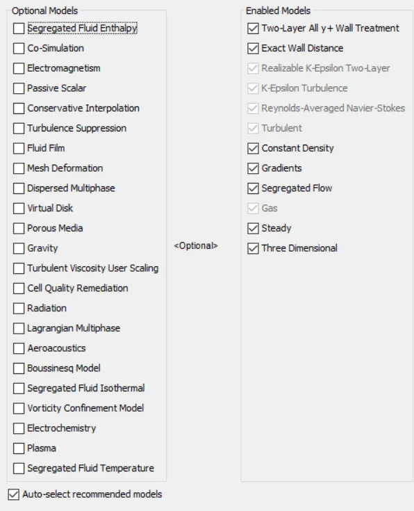
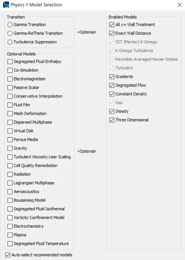
• After selecting Models inlet velocity of 40m/s and pressure outlet value of 0 pascals is given to inlet and outlet region boundaries respectively.
• Drag and Lift report are created from Reports using Force Coefficient. The coordinate drag is in the direction normal to frontal area and for lift, it is normal to the normal of frontal area.
• Density:1.18415 kg/m^3
• Reference Area:0.1150218 m^2
• Reference Velocity:40m/s.

RESULTS

Part 1: Slant Angle 25°

Case I Turbulence Modelling: k-Epsilon

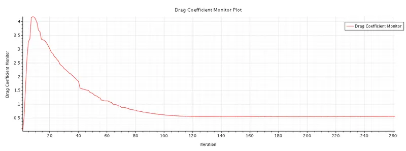
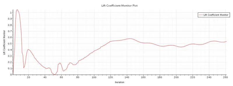
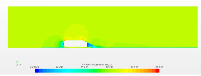
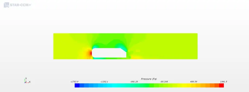
Case II K-Omega

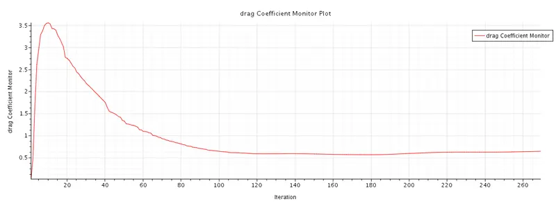
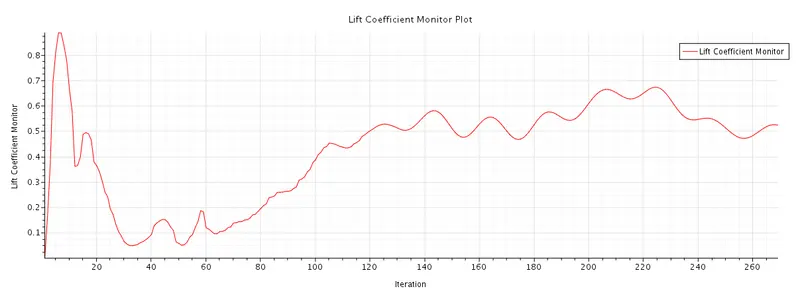
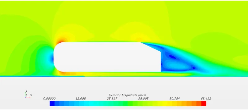
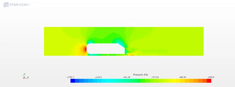
Inference from the above Plots and Contour

• Drag Coefficient for k epsilon case and k-omega case are 0.535 and 0.515 respectively
• Lift Coefficient for k epsilon case and k-omega cases are 0.525 and 0.518.
• The maximum velocity for Case I was 63.246 and for Case II was 63.492
• Both cases showed low velocity at the rear due to recirculation and also the low pressure in the wake region.
• The pressure is high at the front and it due to the impact of a particle on the front sides
• K-Omega capture the physics of flow seperation effectively in comparison to the k-Epsilon

Comparison Between Experimental and Simulation Results

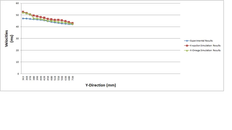
At x :-13

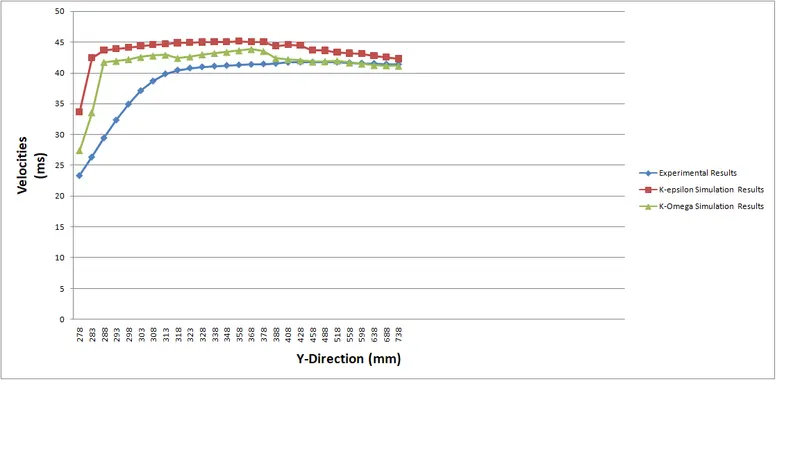
At x:-63

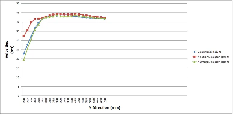
At x:-113

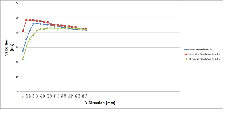
At x:-263

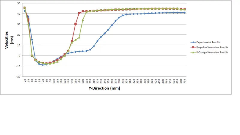
At x: 37

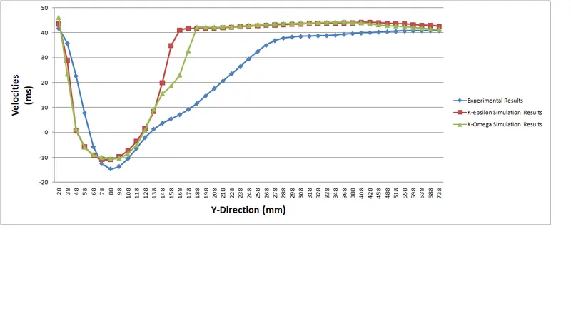
At x : 87

At x : 137

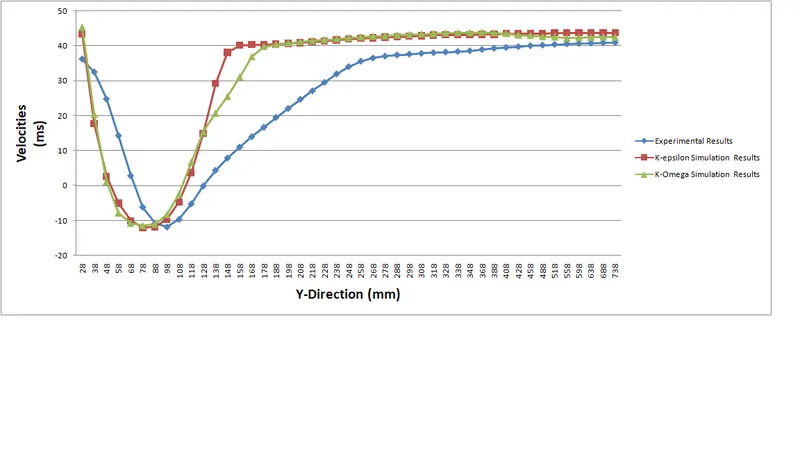
The conclusion that can be drawn is that

• The pattern looks really close to the experimental result profile
• Moreover, the k-omega result pattern is much to experimental result than its counterpart k-epsilon.
• The profiles positive coordinate location of k epsilon k-omega looks similar in pattern but there's a higher percentage of error, the reason could be the coordinates are in the wake region

PART 2 Slant Angle 35

Case I K-Epsilon Model

Case II K-Omega

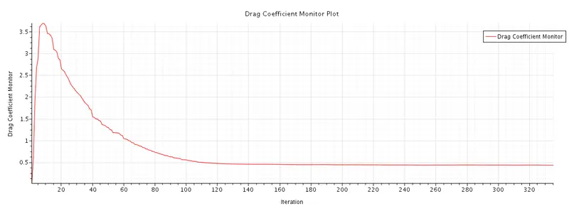
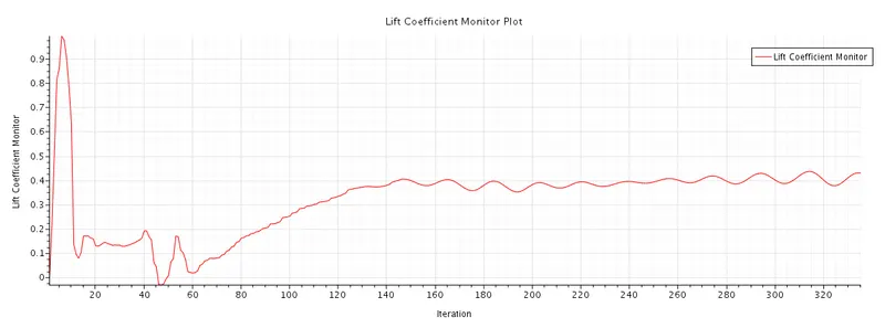
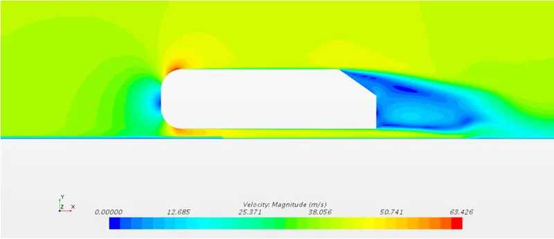
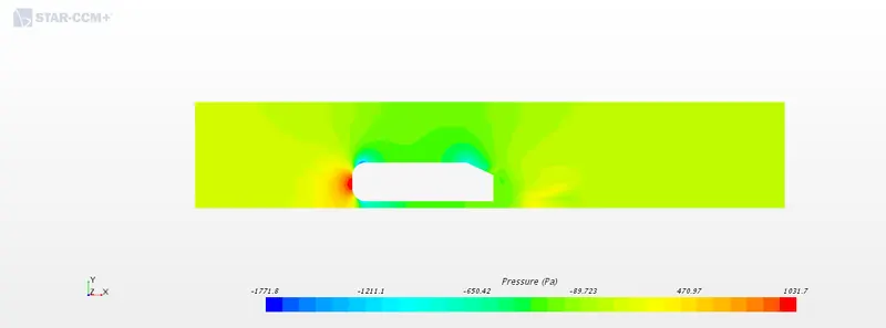
Inference from the above Plots and Contour

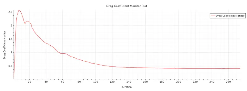
• Drag Coefficient for k epsilon case and k-omega case are 0.445 and 0.417 respectively
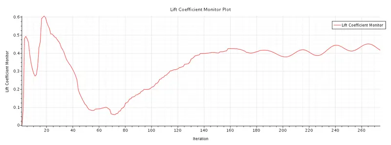
• Lift Coefficient for k epsilon case and k-omega cases are 0.421 and 0.439.
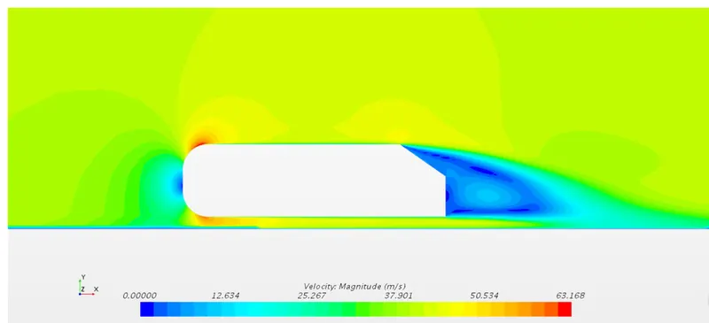
• The maximum velocity for Case I was 63.168 and for Case II was 63.426
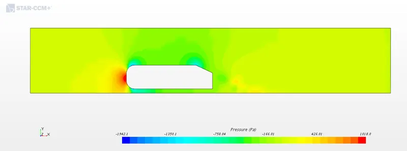
• Both cases showed low velocity at the rear due to recirculation and also the low pressure in the wake region.
• The pressure is high at the front and it due to the impact of a particle on the front sides
• K-Omega capture the physics of flow separation effectively in comparison to the k-Epsilon

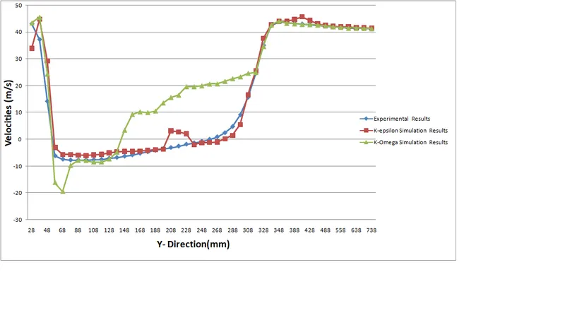
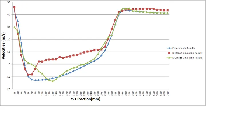
Comparison Between Experimental and Simulation Results

At x = -13mm

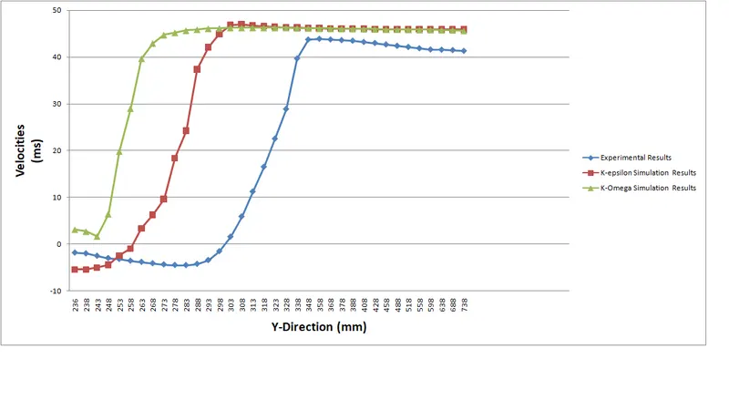
At x = -87mm

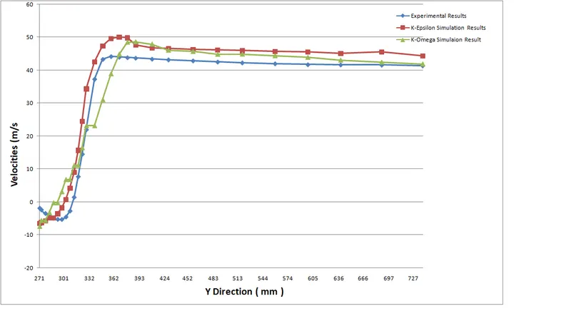
At x = -113mm

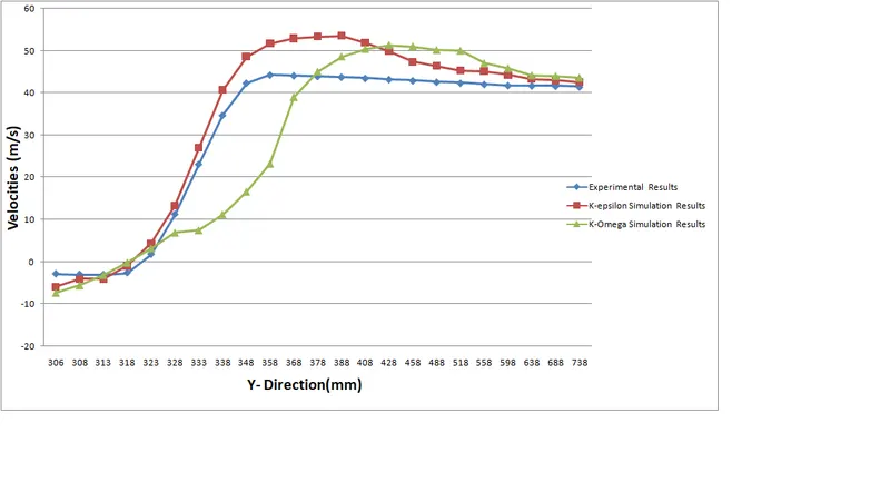
At x = -263mm

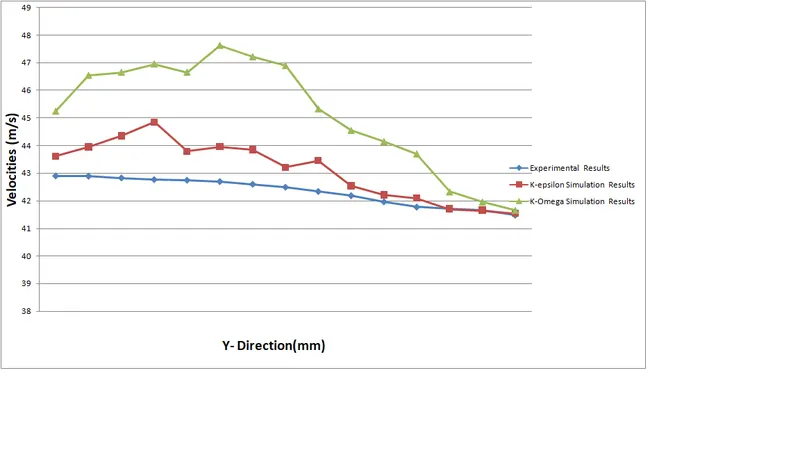
At x = 37mm

At x = 87mm

At x = 137mm

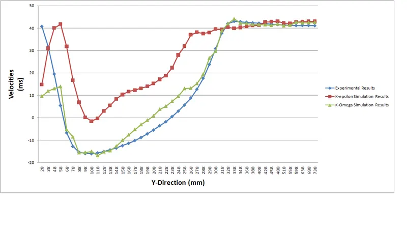
The inference results are quite similar to that of Part I but the mid part of the profile has greater variation but anyhow it can be observed from the last three plots that k-Omega results are pretty closer to that of experimental Results. The above reasons justify that K-Omega is a better option to obtain the result for this challenge