Project 1 : Flow over Ahmed Body

The Ahmed body represents a simplified, ground vehicle geometry of a bluff body type. Its shape is simple enough to allow for accurate flow simulation but retains some important practical features relevant to automobile bodies. This model describes how to calculate the turbulent flow field around a simple car-like geometry using the different Turbulent Flow models.

The Ahmed body is a generic car body (a simplified vehicle model). The airflow around the Ahmed body captures the essential flow features around an automobile and was first defined and characterized in the experimental work of S. R. Ahmed in 1984. Although it has a very simple shape, the Ahmed body allows us to capture characteristic features that are relevant to bodies in the automobile industry.

In this project, external flow analysis on Ahmed Body in STAR-CCM+ is simulate and results are validated by comparing the velocity profiles at different locations with the experimental results done originally. This is done for two geometries with two different slant angles( 25 degrees and 35 degrees) and for two different turbulent models. Also, to calculate the drag coefficient and lift coefficient for all the configurations.

Objective:

• Create the Ahmed Body slant for both 25⁰ and 35⁰
• Run Steady-state implicit coupled flow simulation
• Use the turbulence models K-OmegsSST and k-epsilon
• Validate the velocity profile along the Ahmed body at different points with the experimental data.
• Calculate the cd and cl using the different turbulence.

1. 3D CAD

Ahmed body dimensions

The first step is to create the geometry of Ahmed body in the STAR-CCM+ 3D cad modeler.

The coordinates of the Ahmed body is identical to the experimental data.

Ahmed body end is at x=0. The front end of the Ahmed body is at -1442 mm in the x-direction.

The body is symmetrical along the y-axis.

Simulation procedure is same for all four cases upto meshing. To change the slant angle we need to change slant dimention in sketch.

Sketch :

2D sketch is drawn as per the given dimensions and it is extruded for the given width. The sketch is as follows.

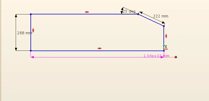
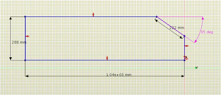
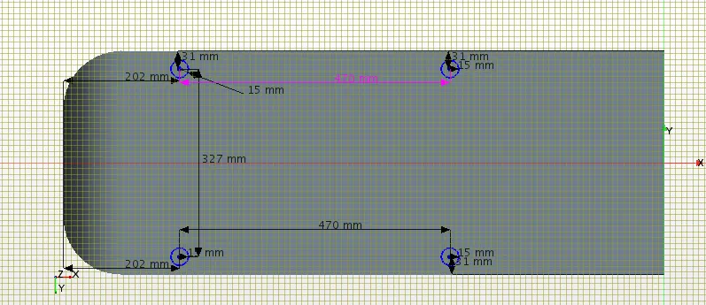
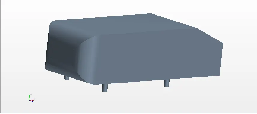
now the above 3D cad body is taken for simulation by creating new geometry part and the Ahmed body appear in a part list. Now windtunnel is created around the body.

Wind tunnel dimensions:

Now we have to create a wind tunnel for external flow analysis. While creating a wind tunnel, we will split the road into two parts, we will use the front part of the road as slip-wall fuction and rest of road is taken as no slip-wall function to achieve proper boundary layer thickness. This can be achive by creating two different blocks and then uniting them. The wind tunnel is ready just name the surfaces as required.

The dimension of windtunnel is 1.5m height, 5m at front till the end of ahmed body and back is of 3m.

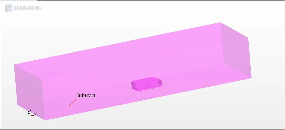
Subtract operation

After creating Ahmed body and the wind tunnel, we will take a CAD to subtract between Ahmed body and wind tunnel to get a nice and clean region for wind flow, without any overlapping surfaces between the Ahmed body legs and wind tunnel.

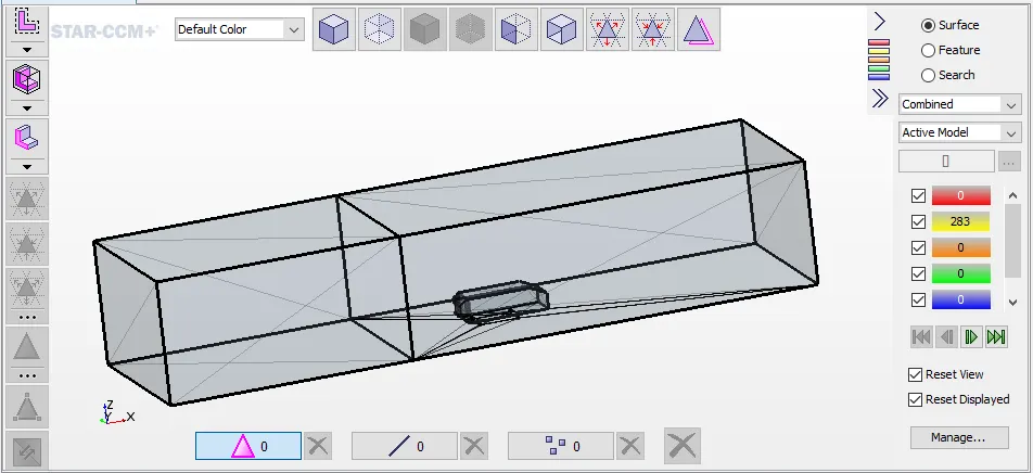
Surface repair:

Once the complete geometry is created, new parts are created from them and some boolean manipulations are done to extract the required volume out of the geometry. Then the part is checked for surface issues and if any, it should be repaired.

Boundary Conditions

• Now we have to assign the subtract part to the region and selecting the option to create a boundary for each part surface and create one region for each part.
• After assigning parts to region we will define the boundary types.
• Inlet: velocity inlet.
• Outlet: pressure outlet.
• Environment (side & top surfaces): symmetry plane.
• Road: wall

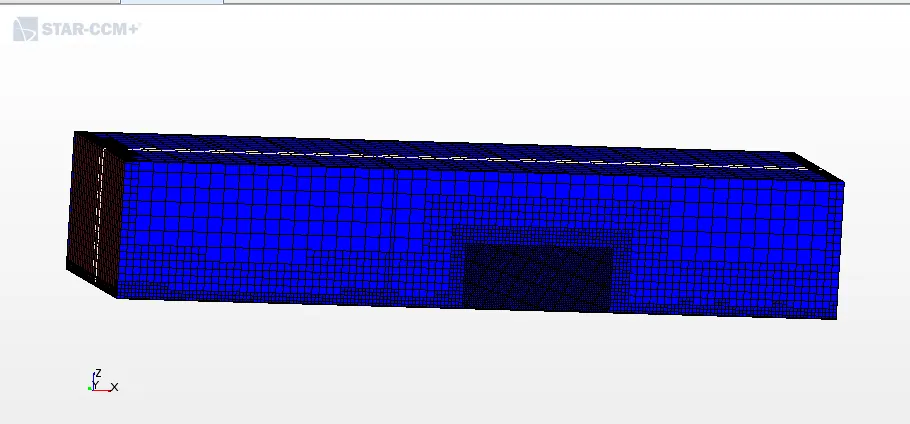
Meshing

Default controls

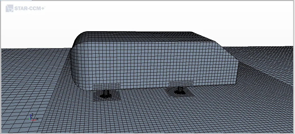
• Base size: 30 mm.
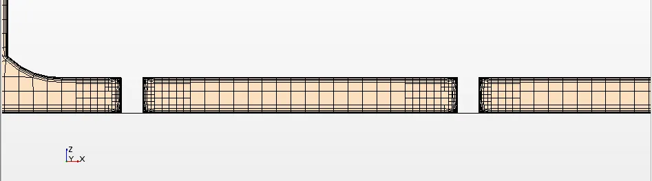
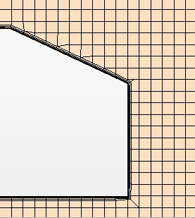
• Number of prism layers: 5.
• Prism layer stretching: 1.5
• Prism layer total thickness: 0.0066 m. (33.33% of base size)

Custome controls

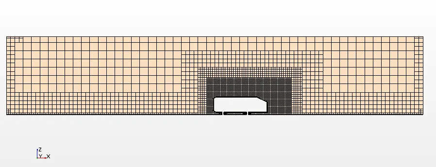
Windtunnel walls = 800% of base Size

Windtunnel Inlet & Outlet = 400 % of base size

Windtunnel base(road) = 200% of base size

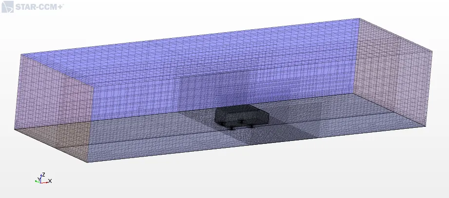
Volumetric control defined on a small block. This block is created for generating a finer mesh near the Ahmed body and to define wake generated by Ahmed body.

• Volumetric control: Cuntomize isotropic size - Enabled.
• Custome size = 100 % relative to base.

Y+ value:

Y plus is an analytical profile covering the viscous sublayer and the buffer layer. In fact, the boundary layer thickness composed of three regions when going far from the wall, started with viscous sublayer, the buffer layer, and the turbulent layer. Y plus is designed to cover only the first two parts and it is expected to be started from the very beginning of the turbulent layer.

For this simulation, it is essential to place the first cell the wall in log-law layer(30 < y+ < 500). So for y+ = 55, the first cell thickness has to be 5 mm for the given velocity, density and viscocity. So the prism layers are generated in a way that the first cell thickness is 5 mm.

Physics setup

The Ahmed body is simulated with two different turbulent model i.e. k-e and k-w SST for two different slant angle of 25 deg and 35 deg. Below shows the relevent simulation model required.

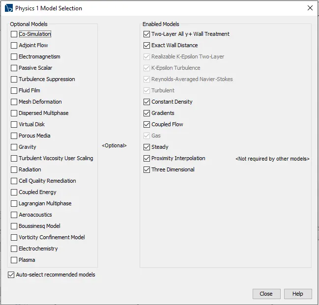
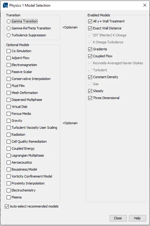
For case I & III For Case II & IV

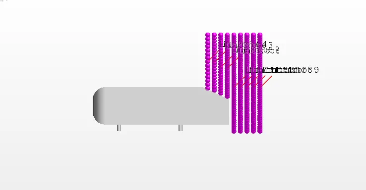
9 probes have been created at different locations on the x-axis to export normalised velocity data.

Case I - Ahmed Body slant 25⁰ for K-e turbulent model

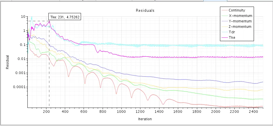
Residuals

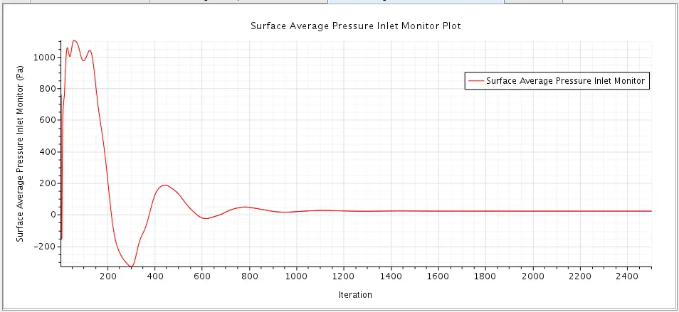
Surface Average inlet Pressure

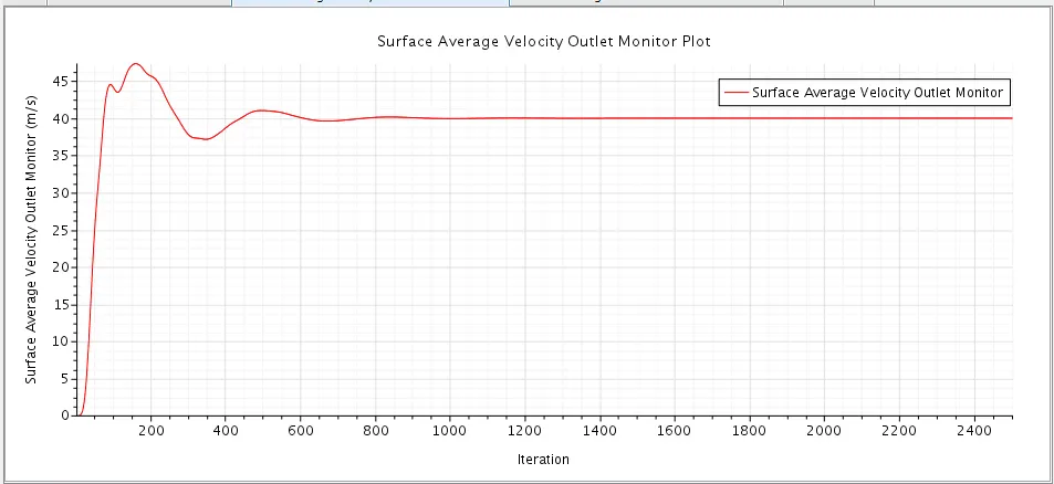
Surface Average Outlet Velocity

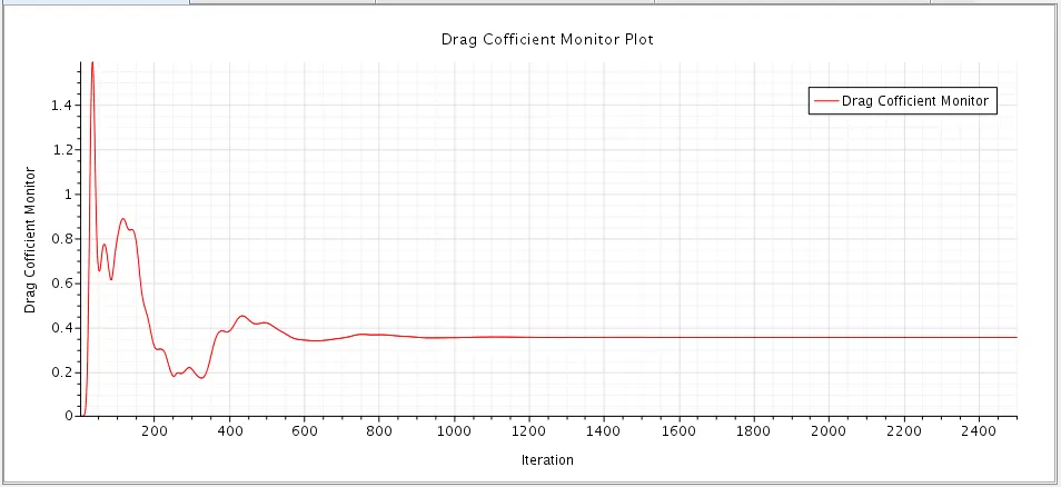
Drag Cofficient

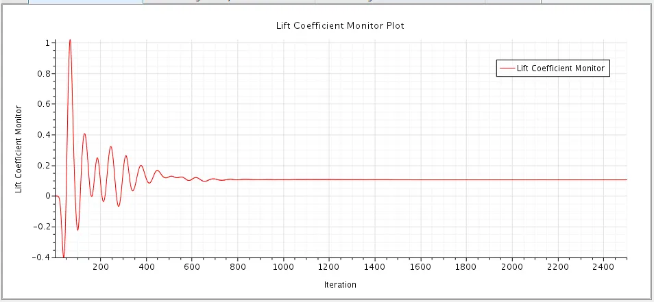
Lift Cofficient

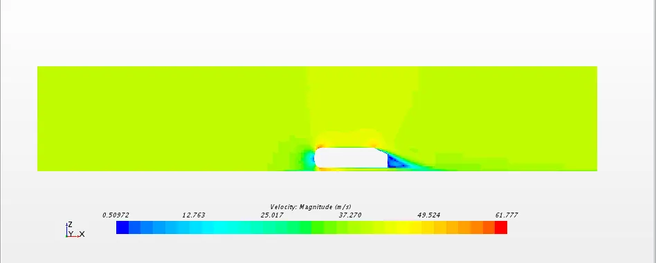
Velocity Contours

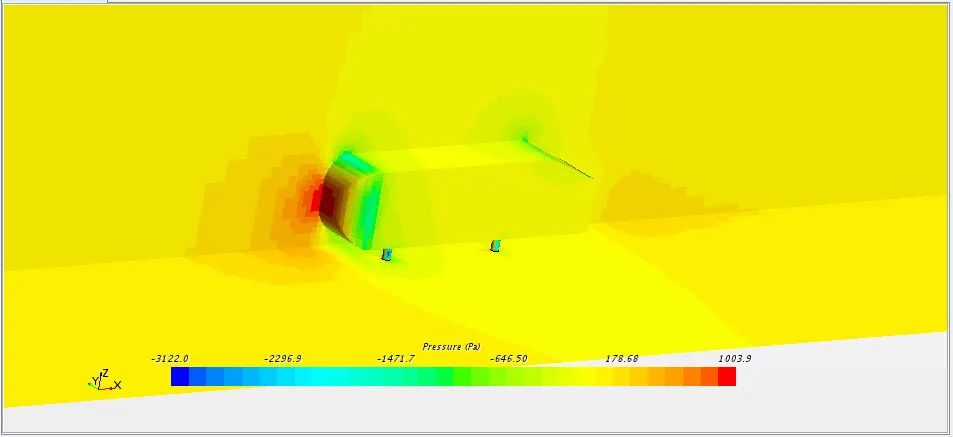
Pressure Contours

Streamlines

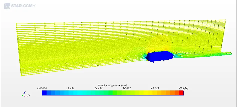
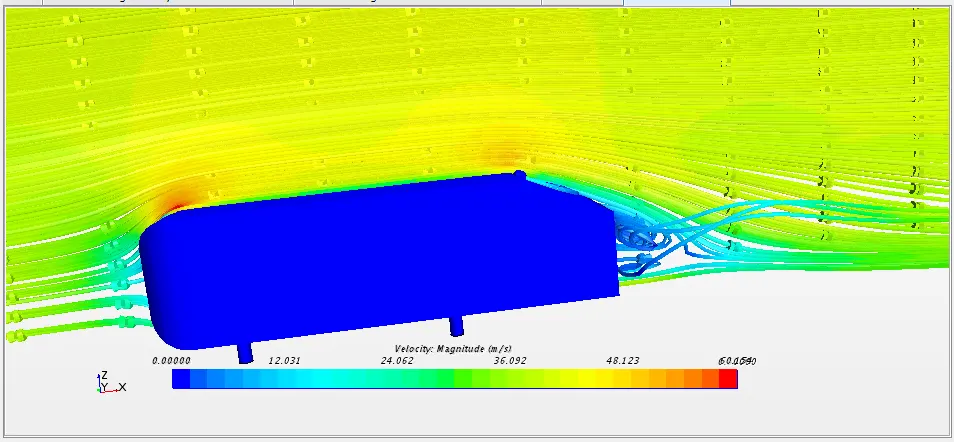
• From the residual plot, surface average inlet pressure and surface average outlet velocity we can see that the solution has converged and reached a steady-state condition.
• Coefficient of Drag: 0.35370750477517304
• Coefficient of Lift: 0.1056237427541368
• From the velocity contour, we can see that the velocity is high at the top region of the Ahmed body at the front of the body. Velocity is low at the back of the Ahmed body at the wake area. Maximum velocity: 61.77 m/s.
• In the pressure contour, we can see that pressure is high at the front face of the Ahmed body due to air impact on a frontal surface of Ahmed body. The pressure is low at the curved region of the Ahmed body where the velocity is high. Maximum pressure:1003.9 Pa

Comparing Simulation Velocity data with Experimental at y = 0

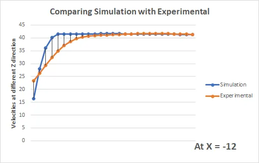
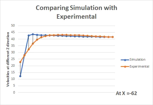
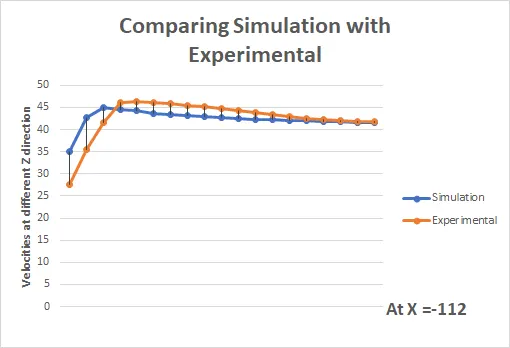
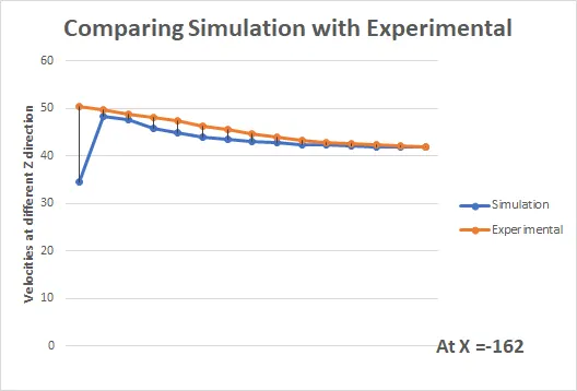
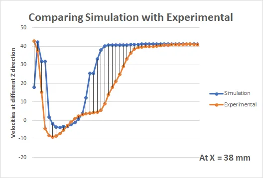
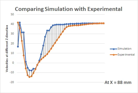
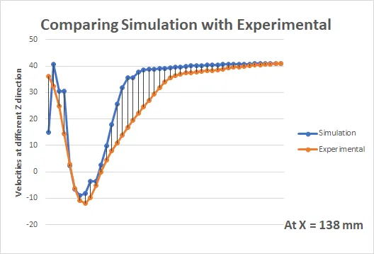
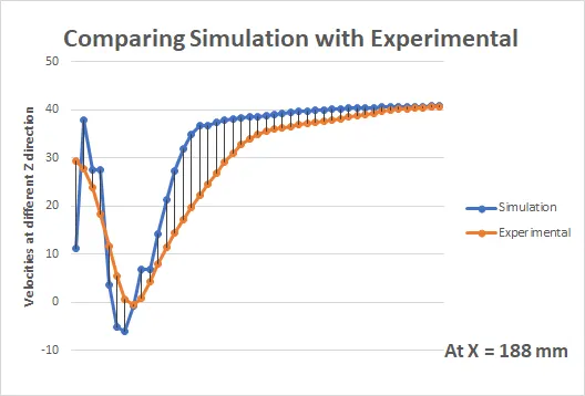
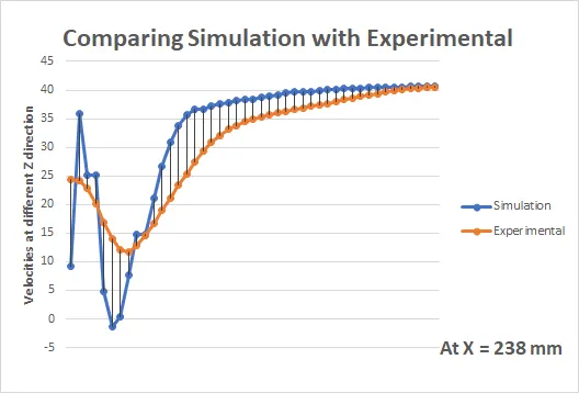
With the help of probes the velocity data is compare at the 9 different location of the region around the ahe Ahmed body which covers the slant and the wake region of Ahmed body. Thus for case I - Ahmed Body slant 25⁰ for K-e turbulent model, first four probes data matches well with the experimental data as it covers the slant of Ahmed body. The other probes are situtated at the wake region formed by Ahmed body and if we see some of velocity data shows higher percentage error.

In all of the 9 we can see that fast few velocities values and last velocities values matches well with the experimental data but the middle values are showing higher % error so this is the effect of selecting a k-e model for defining turbulence.

Case II - Ahmed Body slant 25⁰ for K-w turbulent model

Residuals

Surface Average inlet Pressure

Surface Average Outlet Velocity

Drag Cofficient

Lift Cofficient

Velocity Contours

Pressure Contours

Streamlines

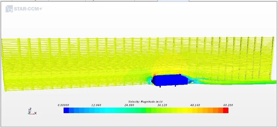
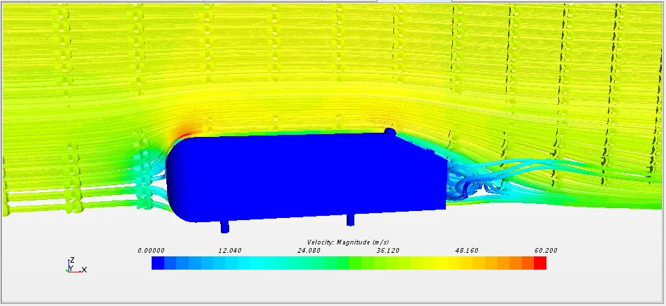
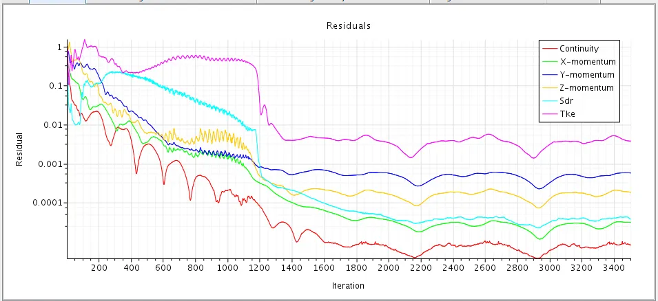
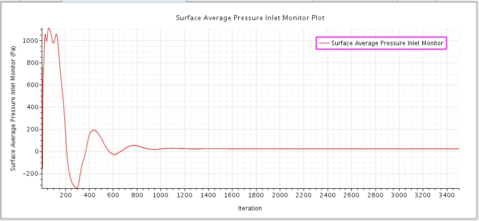
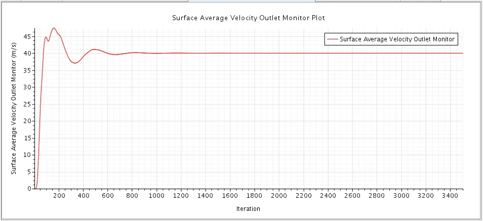
• From the residual plot, surface average inlet pressure and surface average outlet velocity we can see that the solution has converged and reached a steady-state condition.
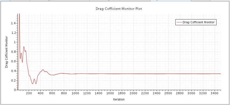
• Coefficient of Drag: 0.33860590323451467
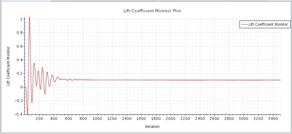
• Coefficient of Lift: 0.1023405787462653
• From the drag and lifft values we can say that for same geometry drag changes from 0.35 to 0.33 this is the effect of selecting k-w turbulence model.
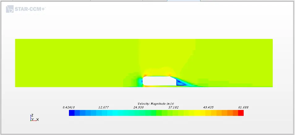
• From the velocity contour, we can see that the velocity is high at the top region of the Ahmed body at the front of the body. Velocity is low at the back of the Ahmed body at the wake area. Maximum velocity: 61.68 m/s.
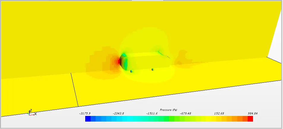
• In the pressure contour, we can see that pressure is high at the front face of the Ahmed body due to air impact on a frontal surface of Ahmed body. The pressure is low at the curved region of the Ahmed body where the velocity is high. Maximum pressure:984.84 Pa

Comparing Simulation Velocity data with Experimental at y = 0

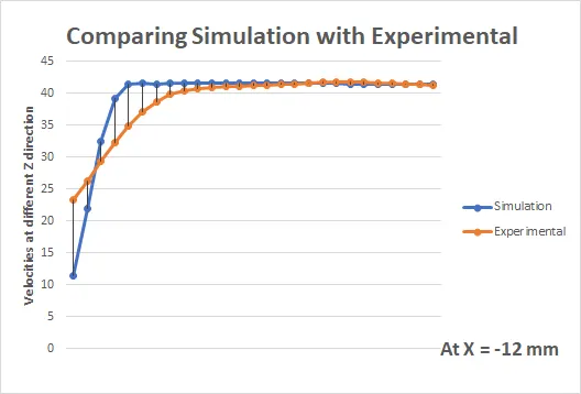
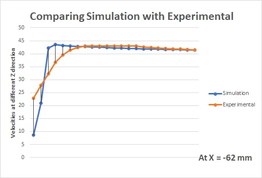
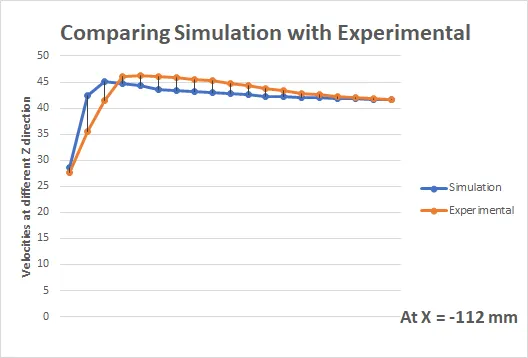
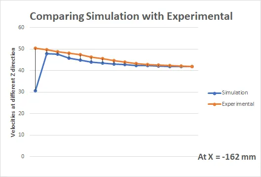
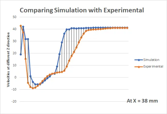
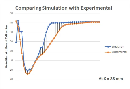
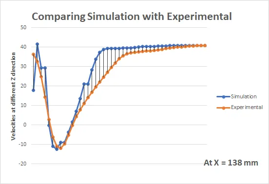
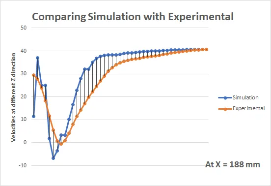
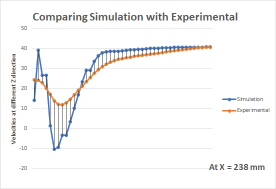
So from all of the above comparision graphs we can see that most of the velocity profile of simulation nearly matches well with the experimental data so from this we can say that k-w model gives better results than k-e model of turbulence.

Case III - Ahmed Body slant 35⁰ for K-e turbulent model

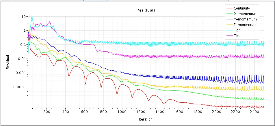
Residuals

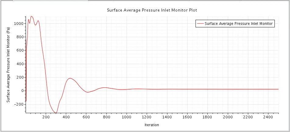
Surface Average inlet Pressure

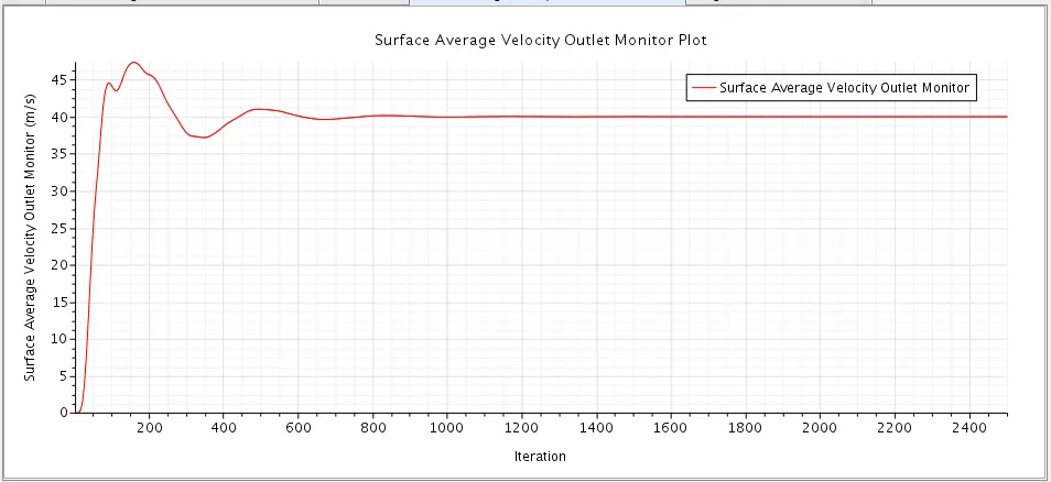
Surface Average Outlet Velocity

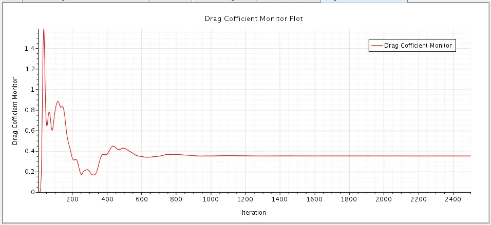
Drag Cofficient

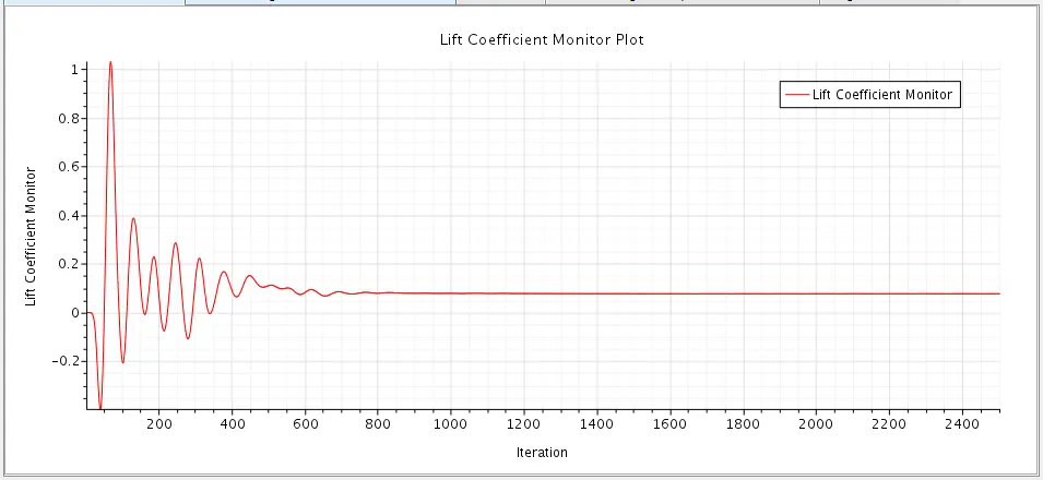
Lift Cofficient

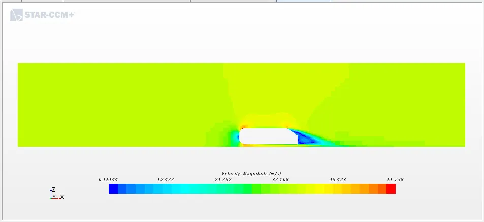
Velocity Contours

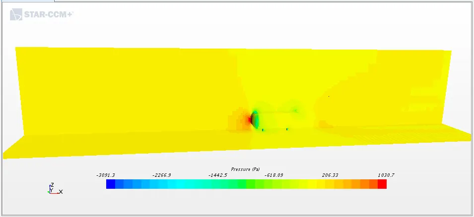
Pressure Contours

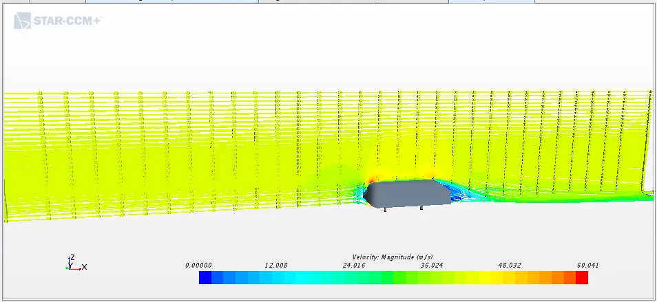
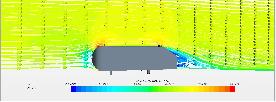
Streamlines

• From the residual plot, surface average inlet pressure and surface average outlet velocity we can see that the solution has converged and reached a steady-state condition.
• Coefficient of Drag: 0.35491952787595316 slightly greater than case I
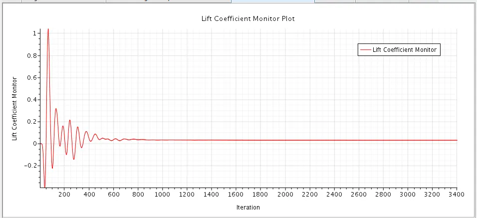
• Coefficient of Lift: 0.0770906109750808 much lesser than case I
• From the velocity contour, we can see that the velocity is high at the top region of the Ahmed body at the front of the body. Velocity is low at the back of the Ahmed body at the wake area. Maximum velocity: 61.73 m/s.
• In the pressure contour, we can see that pressure is high at the front face of the Ahmed body due to air impact on a frontal surface of Ahmed body. The pressure is low at the curved region of the Ahmed body where the velocity is high. Maximum pressure:1030.7 Pa

Comparing Simulation Velocity data with Experimental at y = 0

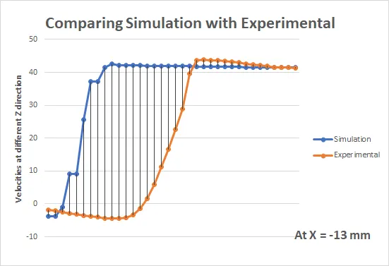
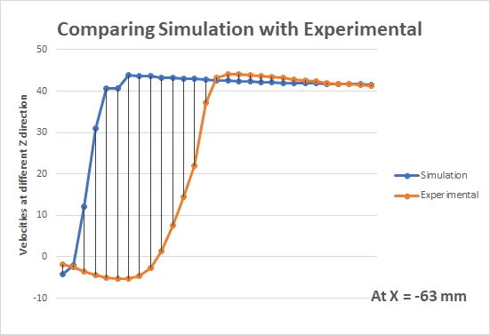
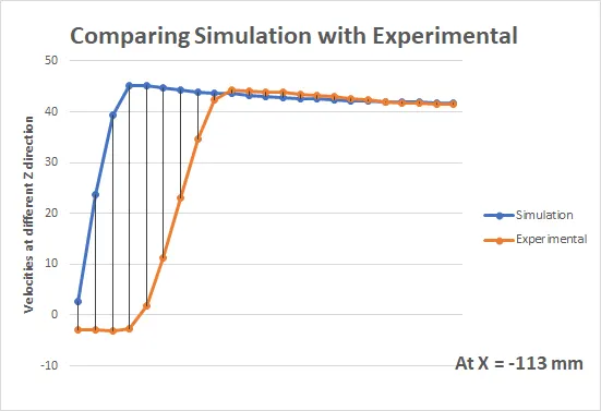
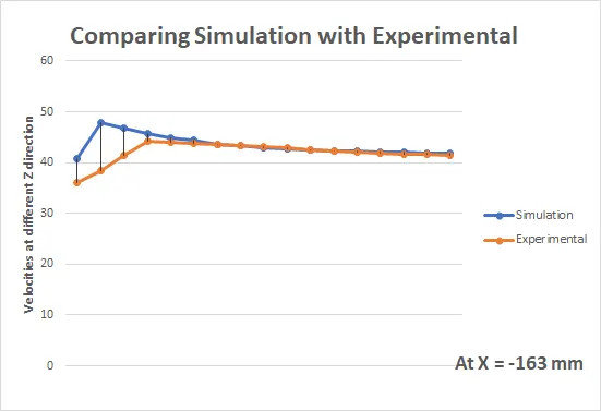
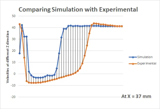
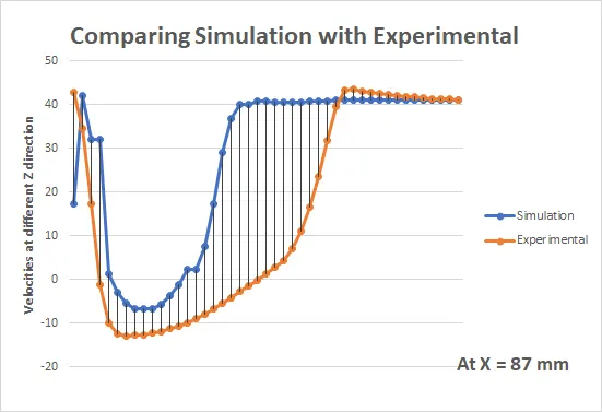
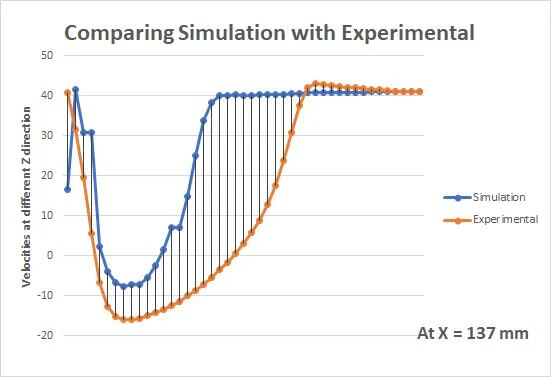
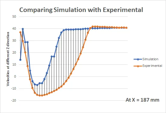
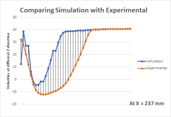
From the graphs we can see tat for all the 9 probes or location data simulation velocity data exactly matches for few starting and for few ending values. The middle velocity values are showing higher %error for matching with experimental data. And the reason is selecting k-e model.

Case IV - Ahmed Body slant 35⁰ for K-w turbulent model

Residuals

Surface Average inlet Pressure

Surface Average Outlet Velocity

Drag Cofficient

Lift Cofficient

Velocity Contours

Pressure Contours

Streamlines

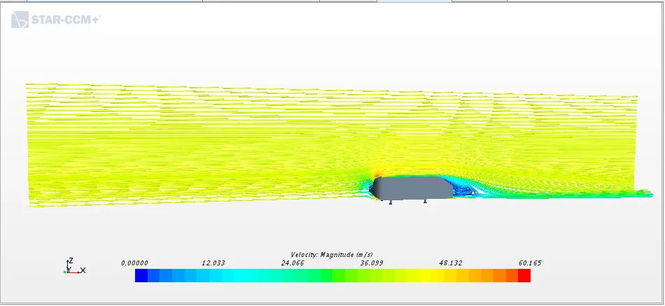
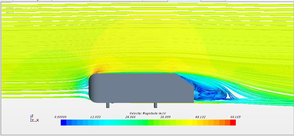
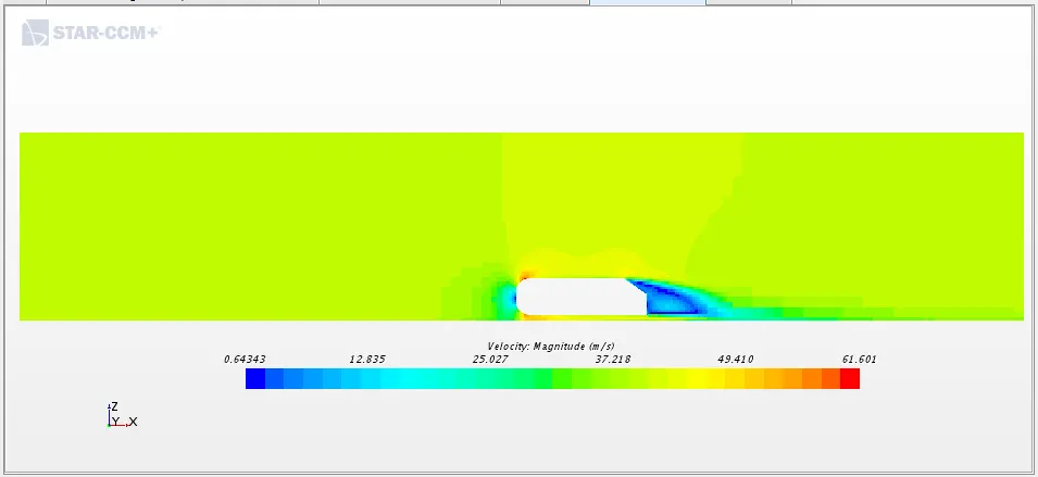
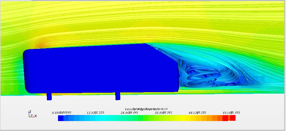
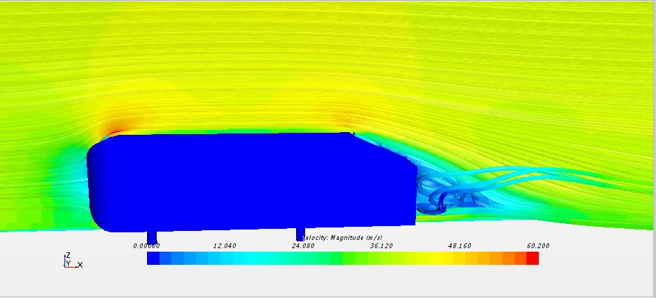
Recirculation seen at the end of body and the vortex is seems detached.

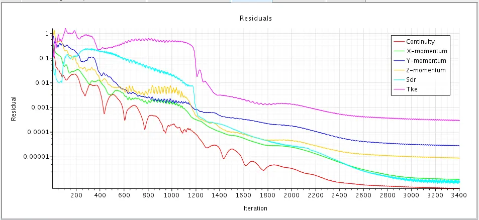
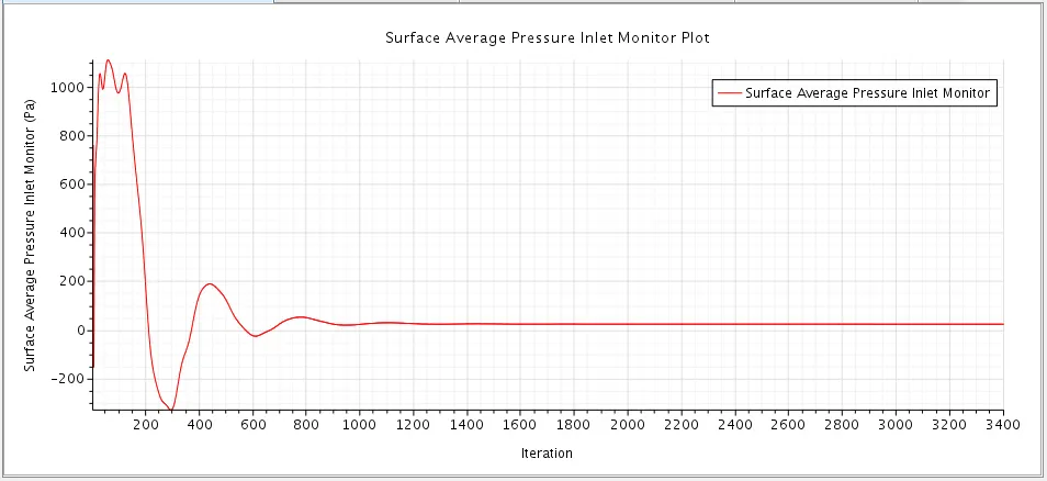
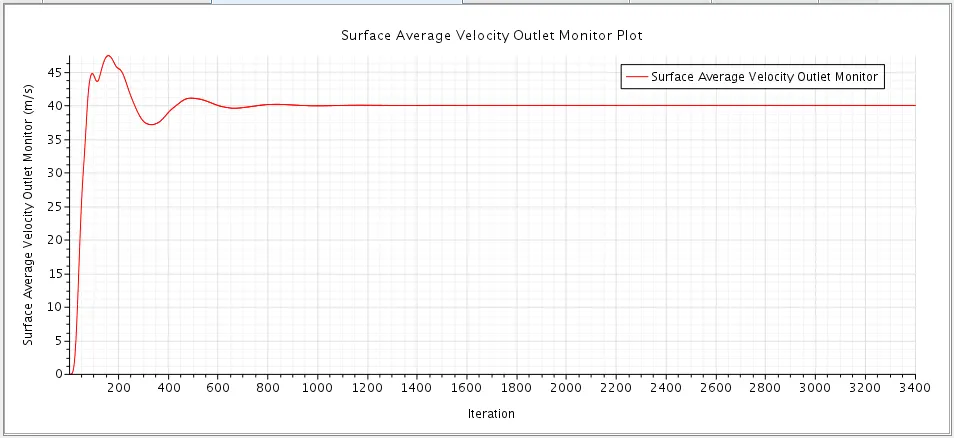
• From the residual plot, surface average inlet pressure and surface average outlet velocity we can see that the solution has converged and reached a steady-state condition.
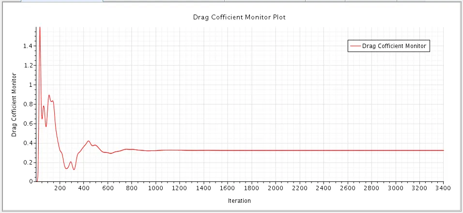
• Coefficient of Drag: 0.3215951213574271
• Coefficient of Lift: 0.030651733691728356
• From the velocity contour, we can see that the velocity is high at the top region of the Ahmed body at the front of the body. Velocity is low at the back of the Ahmed body at the wake area. Maximum velocity: 61.6 m/s.
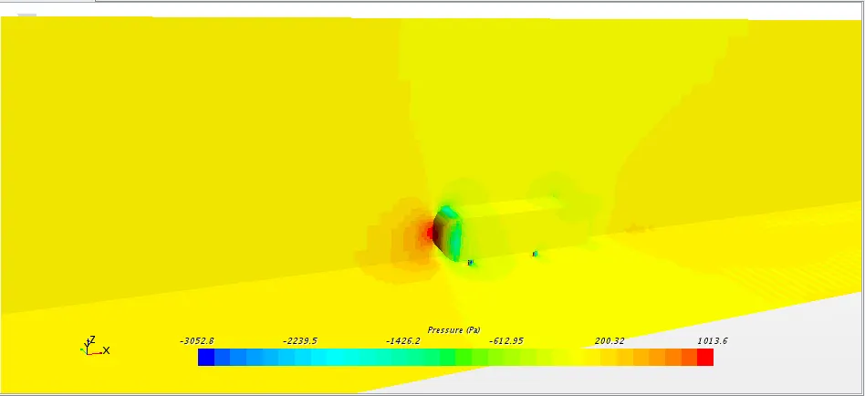
• In the pressure contour, we can see that pressure is high at the front face of the Ahmed body due to air impact on a frontal surface of Ahmed body. The pressure is low at the curved region of the Ahmed body where the velocity is high. Maximum pressure:1013.6 Pa

Comparing Simulation Velocity data with Experimental at y = 0

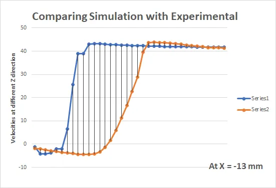
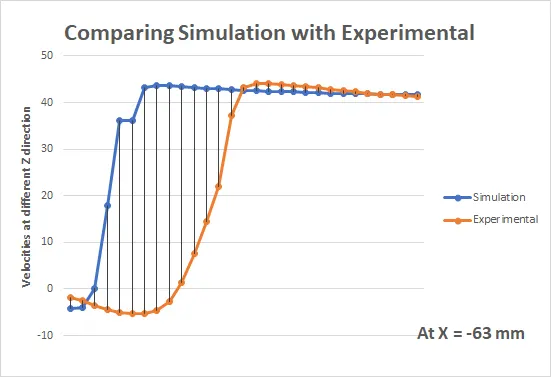
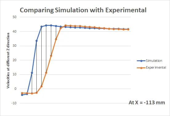
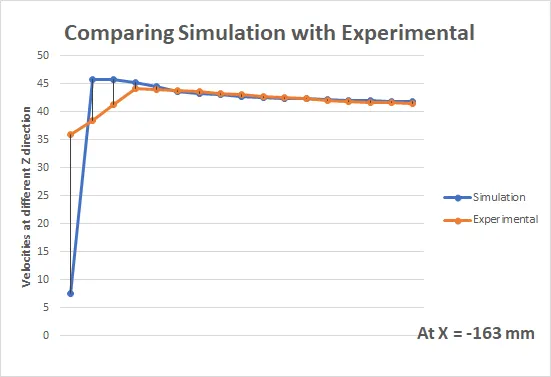
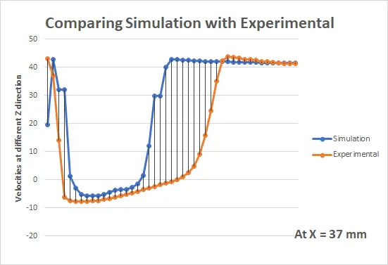
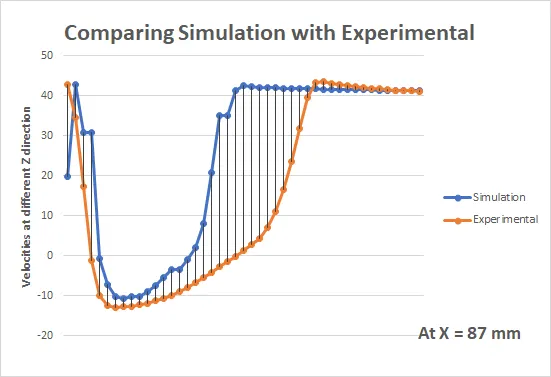
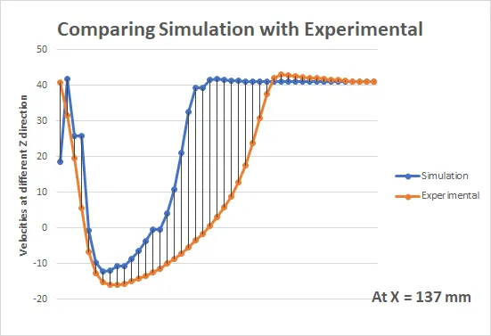
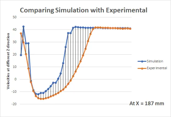
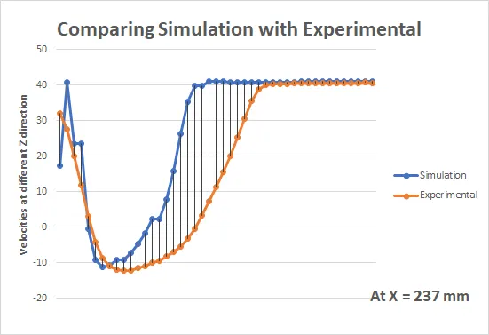
The normalised velocity comparision graphs for case IV shows that k-w model is better for describing flow profile. The experimental and simulation normalised velocities and flow profile are in close proximity with each other

Conclusions

The SST k-omega turbulence model is a two-equation eddy-viscosity model that is used for many aerodynamic applications. It is a hybrid model combining the Wilcox k-omega and the k-epsilon models. A blending function, F1, activates the Wilcox model near the wall and the k-epsilon model in the free stream. The k-omega model is well suited for simulating flow in the viscous sub-layer and the k-epsilon model is ideal for predicting flow behavior in regions away from the wall. As we are comparing normalised velocity data of simumulation with experimental data, the results obtained out of k-w SST model will be more accurate.

Slope angle of the slanted surface have significant effects on the characteristics of the wake flow. Like the vorticity contours on the slanted surface with slant angle = 25 deg is nearly attached to the surface, those which are on the slanted surfaces with slant angle = 35 deg which are more detached. The vortex formed by slant angle = 35 deg is bigger than slant angle = 25 deg.

For alpha = 35

For alpha = 25

From all of the darag cofficient data we can say that due to the flow seperation the drag generated at slant angle a= 35 deg is less than a=25 deg.

The velocity profile on slant is shows a straight line as it is taken on the surface of body and as we move towards positive distance probes we can see a doveloped flow.

The recirculation region captured more accurately by the K-Omega SST model in both the slant angles. This again due to the fact, this algorithm can predict flow separation better than other 2 equation models.