Project 1 - Data Handling and Interpolation

1. Project 1 :

Solve the simple harmonic oscillator equation [m . dx² / dt² = -k.x ] for a given m (mass) and k (spring constant) values using ‘ode45’ and ‘ode23’ solver in MATLAB.

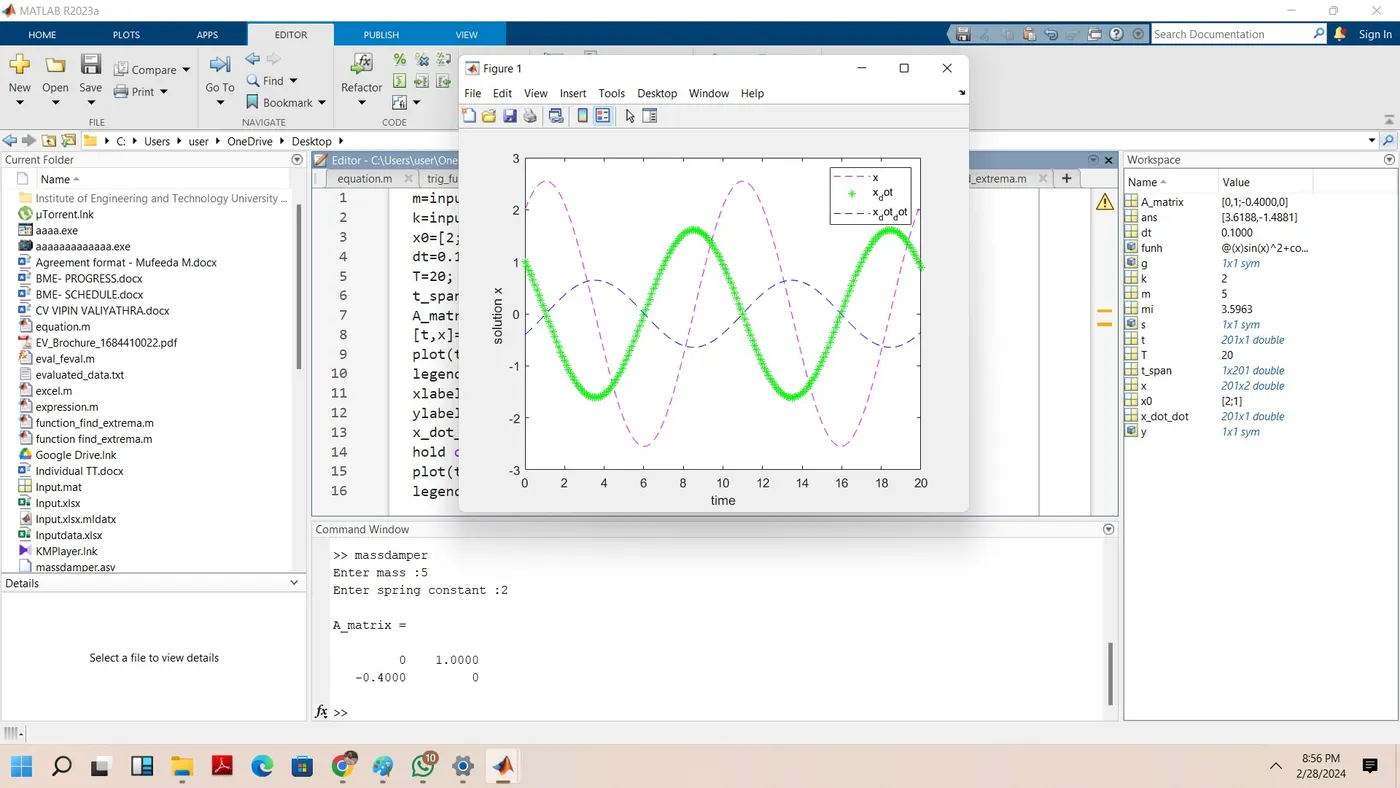
Plot x, x_dot (ẋ) & x_dot_dot (ẍ).

Use the input dialog box to get ‘m’ & ‘k’ values from the user.

Compare ‘ode45’ and ‘ode23’ plots and explain.

Ans

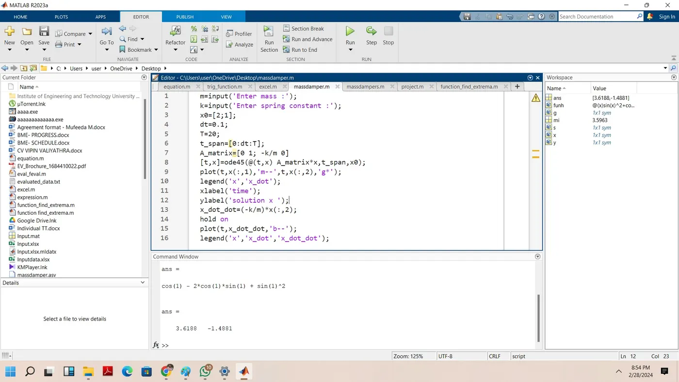
Programme for ode45

m=input('Enter mass :');

k=input('Enter spring constant :');

x0=[2;1];

dt=0.1;

T=20;

t_span=[0:dt:T];

A_matrix=[0 1; -k/m 0]

[t,x]=ode45(@(t,x) A_matrix*x,t_span,x0);

plot(t,x(:,1),'m--',t,x(:,2),'g*');

legend('x','x_dot');

xlabel('time');

ylabel('solution x ');

x_dot_dot=(-k/m)*x(:,2);

hold on

plot(t,x_dot_dot,'b--');

legend('x','x_dot','x_dot_dot');

Programme for ode23

m=input('Enter mass :');

k=input('Enter spring constant :');

x0=[2;1];

dt=0.1;

T=20;

t_span=[0:dt:T];

A_matrix=[0 1; -k/m 0];

[t,x]=ode23(@(t,x) A_matrix*x,t_span,x0);

plot(t,x(:,1),'m--',t,x(:,2),'g*');

legend('x','x_dot');

xlabel('time');

ylabel('solution x ');

x_dot_dot=(-k/m)*x(:,2);

hold on

plot(t,x_dot_dot,'b--');

legend('x','x_dot','x_dot_dot');

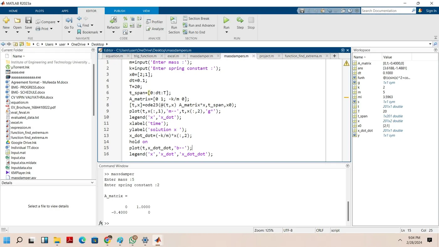
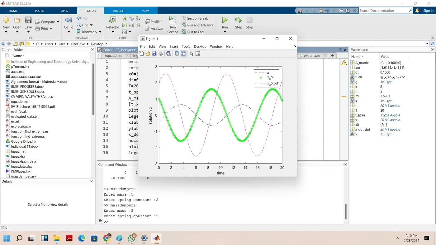
ode23 is a three-stage, third-order, Runge-Kutta method. ode45 is a six-stage, fifth-order, Runge-Kutta method. ode45 does more work per step than ode23, but can take much larger steps. For differential equations with smooth solutions, ode45 is often more accurate than ode23. In this case also ode45 is having better performance from the results shown in screen shoots

2.

Write a program to perform the following steps

load altitude vs temperature data from the tables International Standard Atmosphere (ISA) ((click on the link))

use the ‘polyfit’ function to determine a regression model: T = f(h) for the above table.

evaluate the model determined using the ‘polyval’ function

determine the goodness of fit (goodnessOfFit function)

Generate comparative plot for the loaded and evaluated data

store polyval evaluated data into a text file.

Ans

Programme

K=xlsread('mini_project.xlsx','sheet1','A3:B52');

E=K(:,1);

T=K(:,2);

plot(T,E,'O')

title('Elevation vs Temperature');xlabel('elevation');ylabel('temperature');

a=polyfit(T,E,1)

z=polyval(a,T);

gof = goodnessOfFit(E,T,'MSE');

hold on ;

plot(T,z,'*');legend('polyval analysis');

title('regression analysis ');

evaluated_data = [T',z'];

dlmwrite('evaluated_data.txt', evaluated_data, 'delimiter', '\t', 'precision', '%.4f');

disp('Evaluated data saved to evaluated_data.txt');

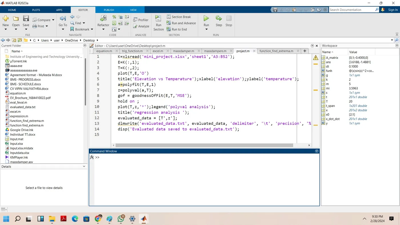
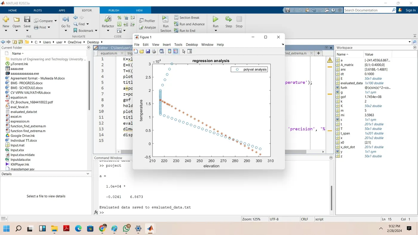
polynomial output is z=-0.0029T+270.6452

3.

Create a function to evaluate the following expression.

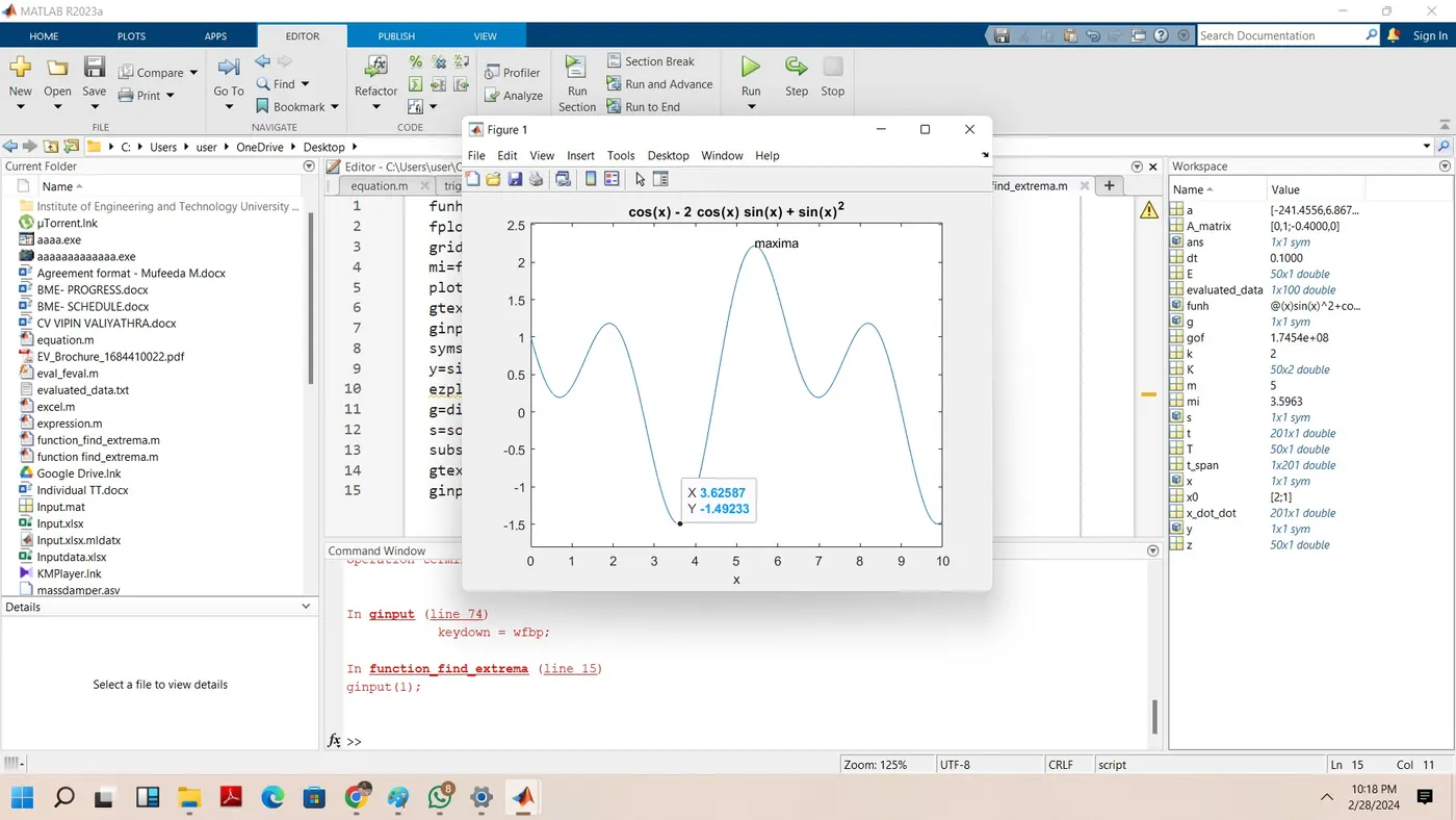
y= sin(x²) +cos(x) - 2 sin(x) cos(x)

Generate the plot and determine all local minima and global maxima values.

Use the ‘gtext’ command to highlight the local minima and global maxima value in the graph.

Hint: make use of 'fminsearch' & 'max' commands.

Ans

funh=@(x) sin(x)^2+cos(x)-2*sin(x)*cos(x);

fplot(funh);

grid on;

mi=fminsearch(funh,2);

plot(mi,funh(mi),'ro','linewidth',5);

gtext('minima');

ginput(1);

syms x;

y=sin(x)^2+cos(x)-2*sin(x)*cos(x);

ezplot(y,[0,10]);

g=diff(y);

s=solve(g);

subs(y,2), subs(y,1)

gtext('maxima');

ginput(1) ;

4.

Project 4 :

Give a brief note on the “contour” command. Illustrate with an example.

Note :

For example, take simple code and execute in MATLAB.

Attach the same along with the answer body.

Ans:

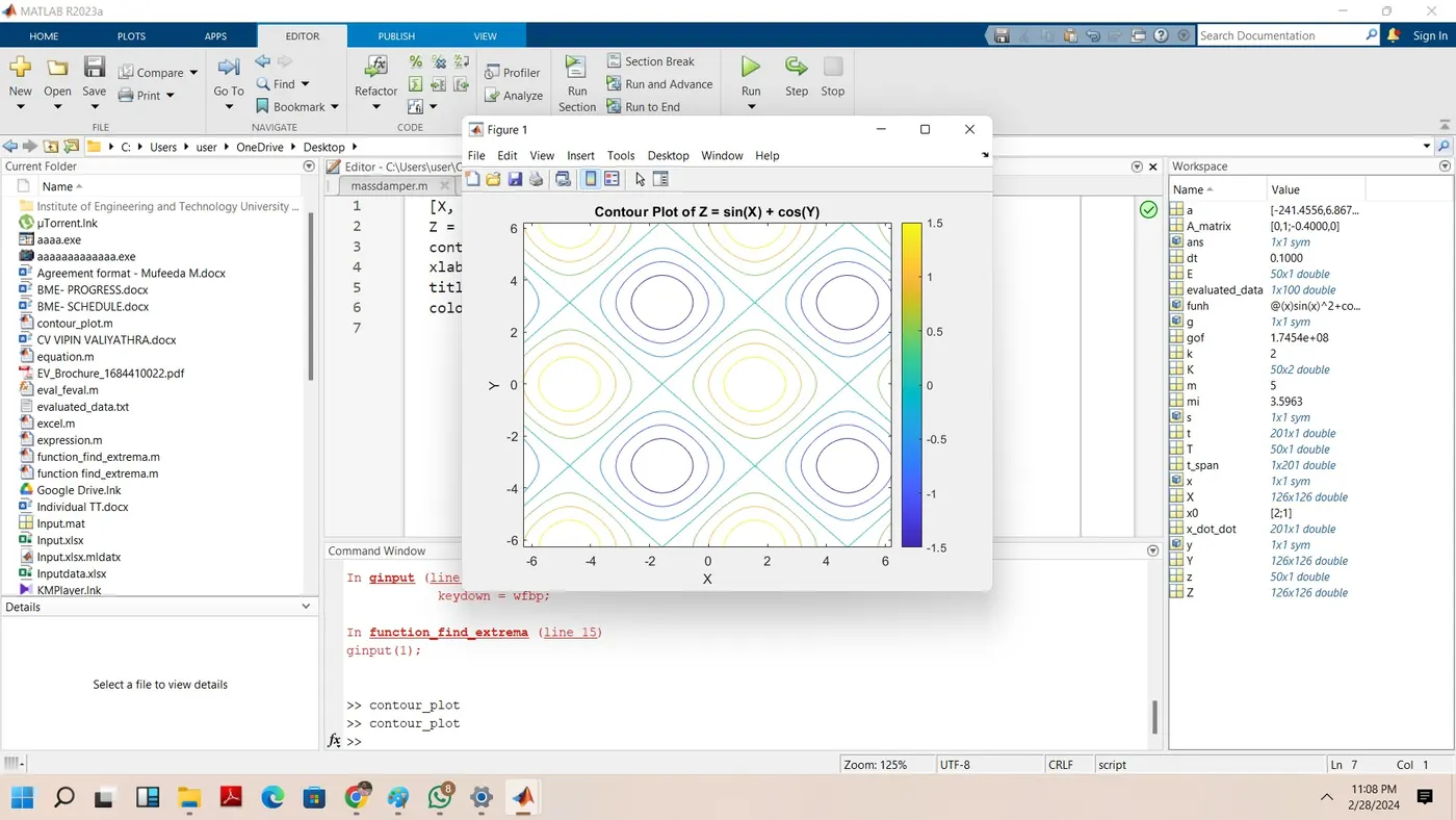
A contour plot is a graphical method to visualize the 3-D surface by plotting constant Z slices called contours in a 2-D format. The contour plot is an alternative to a 3-D surface plot

The contour plot is formed by:

Vertical axis: Independent variable 2

Horizontal axis: Independent variable 1

Lines: iso-response values, can be calculated with the help (x,y).

The independent variable usually restricted to a regular grid. The actual techniques for determining the correct iso-response values are rather complex and almost always computer-generated.

The contour plot is used to depict the change in Z values as compared to X and Y values. If the data (or function) do not form a regular grid, you typically need to perform a 2-D interpolation to form a regular grid.

For one variable data, a run sequence/ histogram is considered necessary. For two-variable data, a scatter plot is considered necessary. The contour plots can also polar co-ordinates (r,theta) instead of traditional rectangular (x, y, z) coordinates.

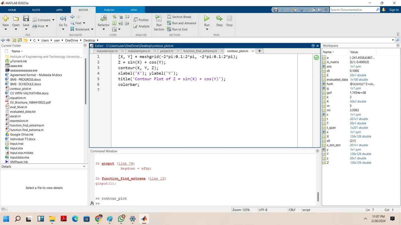
Eg: Contour plot for plotting function Z = Sin (X) + Cos (Y)

[X, Y] = meshgrid(-2*pi:0.1:2*pi, -2*pi:0.1:2*pi);

Z = sin(X) + cos(Y);

contour(X, Y, Z);

xlabel('X'); ylabel('Y');

title('Contour Plot of Z = sin(X) + cos(Y)');

colorbar;