Project 1 - Data Handling and Interpolation
PROJECT (01) -
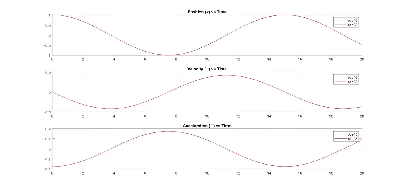
Solving the simple harmonic oscillator equation in MATLAB using the 'ode45' and 'ode23' solvers involves defining the equation and integrating it over time to obtain the position ('x'), velocity ('ẋ'), and acceleration ('ẍ').
Code -
% Ask for user input for mass (m) and spring constant (k)
m = inputdlg('Enter mass (m): ');
m = str2double(m{1}); % Convert the input to a numerical value
k = inputdlg('Enter spring constant (k): ');
k = str2double(k{1}); % Convert the input to a numerical value
% Define the simple harmonic oscillator equation
f = @(t, y) [y(2); -(k/m) * y(1)];
% Set initial conditions
tspan = [0 20]; % Time span for simulation
y0 = [1; 0]; % Initial position and velocity
% Solve using 'ode45'
[t_ode45, sol_ode45] = ode45(f, tspan, y0);
% Solve using 'ode23'
[t_ode23, sol_ode23] = ode23(f, tspan, y0);
% Plotting
figure;
subplot(3,1,1);
plot(t_ode45, sol_ode45(:, 1), 'b', t_ode23, sol_ode23(:, 1), 'r');
title('Position (x) vs Time');
legend('ode45', 'ode23');
subplot(3,1,2);
plot(t_ode45, sol_ode45(:, 2), 'b', t_ode23, sol_ode23(:, 2), 'r');
title('Velocity (ẋ) vs Time');
legend('ode45', 'ode23');
subplot(3,1,3);
accel_ode45 = -(k/m) * sol_ode45(:, 1); % Calculate acceleration
accel_ode23 = -(k/m) * sol_ode23(:, 1);
plot(t_ode45, accel_ode45, 'b', t_ode23, accel_ode23, 'r');
title('Acceleration (ẍ) vs Time');
legend('ode45', 'ode23');
Note that; This code sets up the differential equation, solves it using 'ode45' and 'ode23' for the given time span, and then plots the results for position ('x'), velocity ('ẋ'), and acceleration ('ẍ').
The main difference between 'ode45' and 'ode23' lies in their algorithms for solving ordinary differential equations. 'ode45' is typically more accurate but might be slower, while 'ode23' is less accurate but faster in some cases. The comparison of plots will showcase these differences in accuracy and computational speed.
Feel free to run this code in MATLAB, input your desired 'm' and 'k' values, and observe the plotted results to understand the behavior of the simple harmonic oscillator using these solvers.
Results -
Results for a mass of 4 kgs and spring constant of 0.7 N/m.
PROJECT (04) -
Code -
% Define the function and create a grid of x and y values
[x, y] = meshgrid(-2:0.1:2, -2:0.1:2);
z = x.^2 + y.^2; % Function: f(x, y) = x^2 + y^2
% Plot the contour
contour(x, y, z);
title('Contour Plot of f(x, y) = x^2 + y^2');
xlabel('x');
ylabel('y');
colorbar; % Display the colorbar showing function values
Explaination -
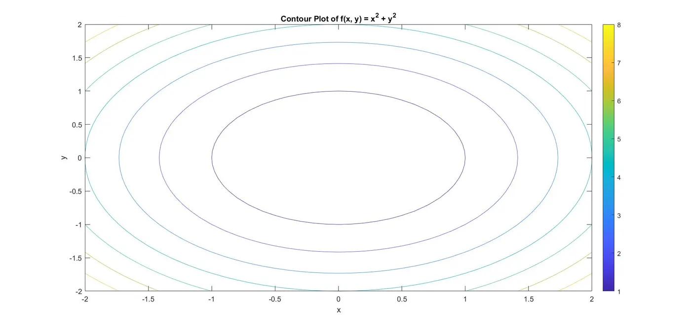
The `contour` command in MATLAB is used to create contour plots, which display the contours or level curves of a function of two variables in a 2D plot. These plots represent the values of the function as curves of constant value. In the above example - - `meshgrid` creates a grid of x and y values ranging from -2 to 2 with an interval of 0.1. - `z` calculates the function values ( f(x, y) = x^2 + y^2 ) for each combination of x and y. - `contour` creates the contour plot using the x, y grid and their corresponding function values. The contour plot displays curves where the function ( f(x, y) = x^2 + y^2 ) takes constant values. Each contour line represents a constant value of the function, and the color variation or labeling shows the different levels of the function values. Adjusting the range or function in the `z` calculation will result in different contour plots representing various functions or landscapes in the (x, y) plane.
Results -
PROJECT (02) -
Code -
% Altitude vs Temperature Data
altitude = [-2000; -1500; -1000; -500; 0; 500; 1000; 1500; 2000; 2500; 3000; 3500; ...
4000; 4500; 5000; 5500; 6000; 6500; 7000; 7500; 8000; 8500; 9000; 9500; ...
10000; 10500; 11000; 11500; 12000; 12500; 13000; 13500; 14000; 14500; ...
15000; 15500; 16000; 16500; 17000; 17500; 18000; 18500; 19000; 19500; ...
20000; 22000; 24000; 26000; 28000; 30000];
temperature = [301.2; 297.9; 294.7; 291.4; 288.15; 284.9; 281.7; 278.4; 275.2; ...
271.9; 268.7; 265.4; 262.2; 258.9; 255.7; 252.4; 249.2; 245.9; 242.7; 239.5; ...
236.2; 233; 229.7; 226.5; 223.3; 220; 216.8; 216.7; 216.7; 216.7; 216.7; ...
216.7; 216.7; 216.7; 216.7; 216.7; 216.7; 216.7; 216.7; 216.7; 216.7; ...
216.7; 216.7; 216.7; 216.7; 218.6; 220.6; 222.5; 224.5; 226.5];
% Using polyfit to determine the regression model
degree = 3; % You can adjust the degree of the polynomial fit
coefficients = polyfit(altitude, temperature, degree);
% Evaluate the model
altitude_range = min(altitude):100:max(altitude); % Define a range for evaluation
evaluated_temperature = polyval(coefficients, altitude_range);
% Goodness of fit
fitted_values = polyval(coefficients, altitude);
goodness = goodnessOfFit(temperature, fitted_values, 'MSE'); % Mean Squared Error
% Generate comparative plot
figure;
plot(altitude, temperature, 'o', altitude_range, evaluated_temperature, '-');
xlabel('Altitude (m)');
ylabel('Temperature (K)');
legend('Loaded Data', 'Evaluated Data');
title('Altitude vs Temperature');
% Store polyval evaluated data into a text file
evaluated_data = [altitude_range; evaluated_temperature];
dlmwrite('evaluated_data.txt', evaluated_data', 'delimiter', '\t');
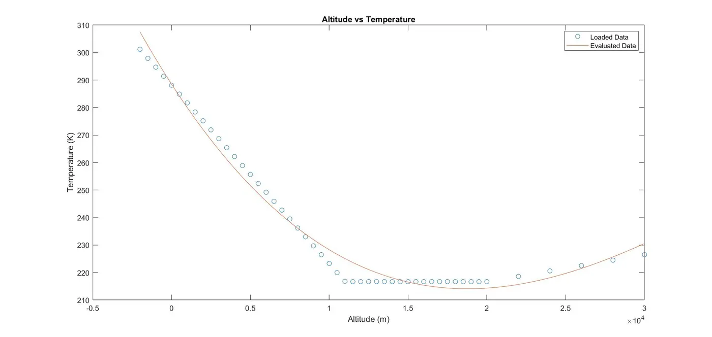
Plot -
PROJECT (03) -
Code -
% Define the function
y_function = @(x) sin(x.^2) + cos(x) - 2 * sin(x) .* cos(x);
% Generate the plot
x_values = linspace(-5, 5, 1000); % Adjust the range as needed
y_values = y_function(x_values);
figure;
plot(x_values, y_values);
xlabel('x');
ylabel('y = sin(x^2) + cos(x) - 2*sin(x)*cos(x)');
title('Plot of the Function');
hold on;
% Use fminsearch to find local minima
local_minima = fminsearch(y_function, 0);
plot(local_minima, y_function(local_minima), 'ro'); % Plot local minima points
gtext(['Local Minima at (x,y) = (', num2str(local_minima), ',', num2str(y_function(local_minima)), ')']);
% Use max function to find global maxima
global_maxima = fminsearch(@(x) -y_function(x), 0); % Minimize the negative of the function for maxima
plot(global_maxima, y_function(global_maxima), 'go'); % Plot global maxima points
gtext(['Global Maxima at (x,y) = (', num2str(global_maxima), ',', num2str(y_function(global_maxima)), ')']);
hold off;
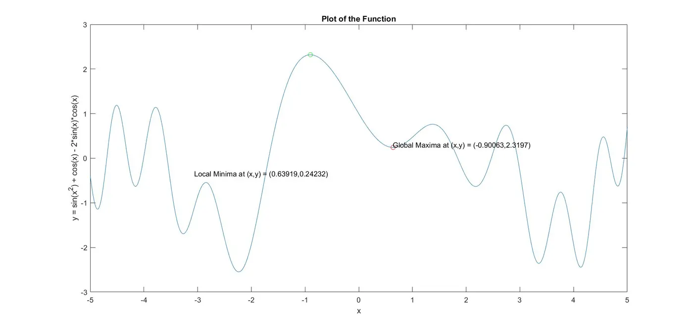
Explaination-
This script defines the function y_function generates a plot of the function within a specified range, uses fminsearch to find local minima and the negative of the function to find the global maxima, and finally, highlights these points on the graph using gtext. Adjust the range in linspace according to your preference.