Project 1 - Data Handling and Interpolation
PROJECT 1:
% Step 1: Get 'm' and 'k' values from the user using input dialog box.
prompt = {'Enter mass (m):', 'Enter spring constant (k):'};
dlgtitle = 'Input for Simple Harmonic Oscillator';
dims = [1 35];
definput = {'1', '1'};
answer = inputdlg(prompt, dlgtitle, dims, definput);
m = str2double(answer{1});
k = str2double(answer{2});
% Step 2: Define the differential equation and initial conditions.
ode = @(t, y) [y(2); -k/m * y(1)]; % dx/dt = y(2), d^2x/dt^2 = -k/m * x
initial_conditions = [1; 0]; % Initial position and velocity
% Step 3: Solve the equation using 'ode45' and 'ode23'.
tspan = [0 10]; % Time span for the simulation
[t_ode45, y_ode45] = ode45(ode, tspan, initial_conditions);
[t_ode23, y_ode23] = ode23(ode, tspan, initial_conditions);
% Step 4: Plot the results.
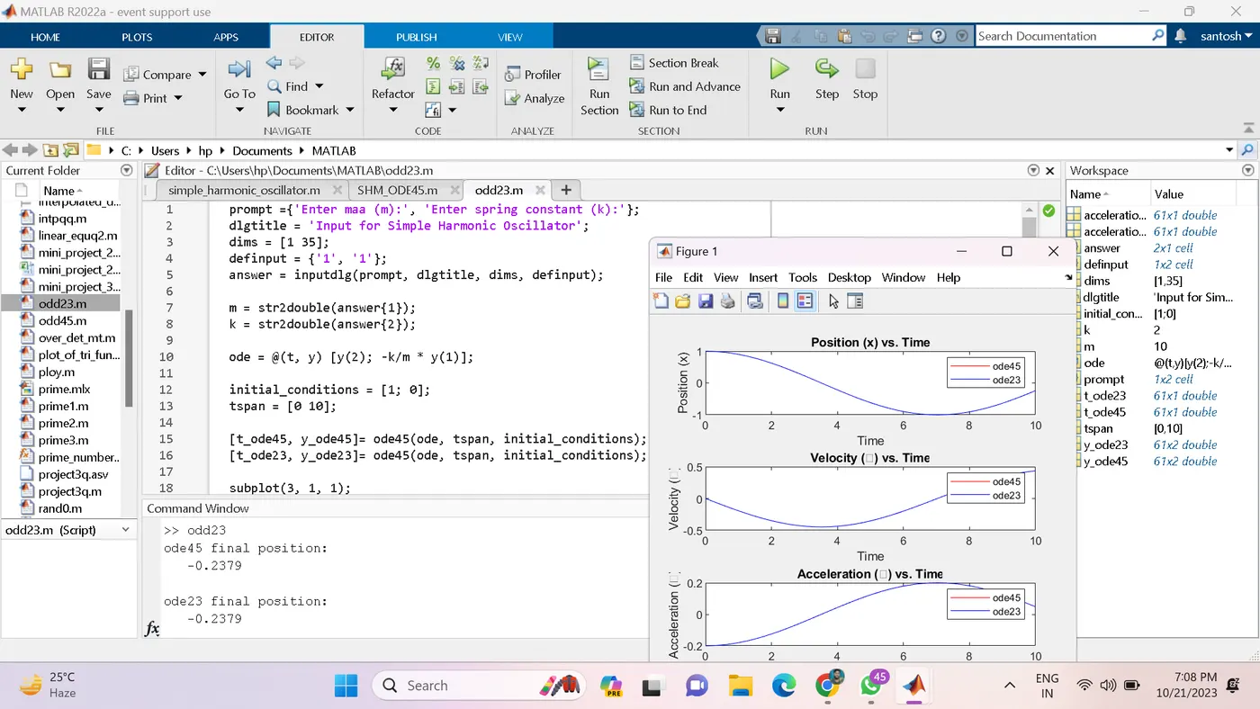
subplot(3, 1, 1);
plot(t_ode45, y_ode45(:, 1), 'r', t_ode23, y_ode23(:, 1), 'b');
title('Position (x) vs. Time');
xlabel('Time');
ylabel('Position (x)');
legend('ode45', 'ode23');
subplot(3, 1, 2);
plot(t_ode45, y_ode45(:, 2), 'r', t_ode23, y_ode23(:, 2), 'b');
title('Velocity (ẋ) vs. Time');
xlabel('Time');
ylabel('Velocity (ẋ)');
legend('ode45', 'ode23');
subplot(3, 1, 3);
acceleration_ode45 = -k/m * y_ode45(:, 1);
acceleration_ode23 = -k/m * y_ode23(:, 1);
plot(t_ode45, acceleration_ode45, 'r', t_ode23, acceleration_ode23, 'b');
title('Acceleration (ẍ) vs. Time');
xlabel('Time');
ylabel('Acceleration (ẍ)');
legend('ode45', 'ode23');
% Step 5: Compare and explain the differences between 'ode45' and 'ode23'.
disp('ode45 final position:');
disp(y_ode45(end, 1));
disp('ode23 final position:');
disp(y_ode23(end, 1));
PROJECT 2
% Load your data into MATLAB
data = xlsread('mini_project_2.xlsx');
altitude = data(:, 1); % Assuming altitude is in the first column
temperature = data(:, 2); % Assuming temperature is in the second column
degree = 2;
coefficients = polyfit(altitude, temperature, degree);
%fine a range of altitudes or specific altitudes of interest
altitude_range = linspace(min(altitude), max(altitude), 100); % Example: 100 points between min and max altitudes
predicted_temperatures = polyval(coefficients, altitude_range);
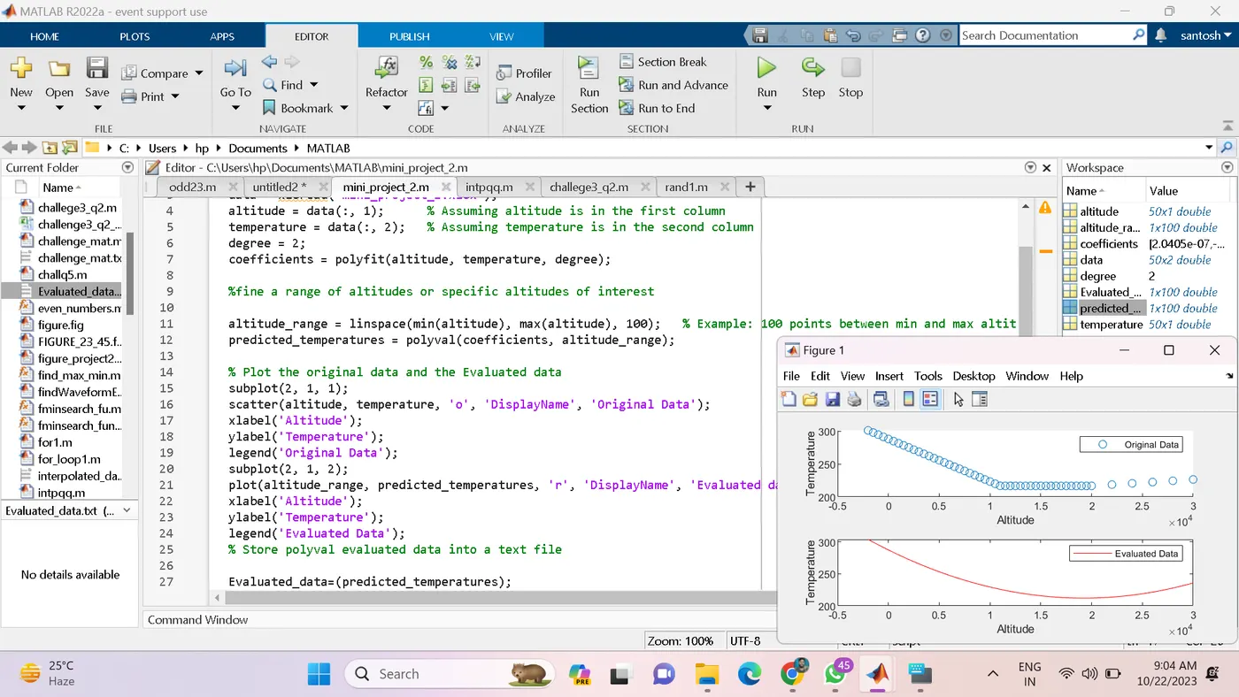
% Plot the original data and the Evaluated data
subplot(2, 1, 1);
scatter(altitude, temperature, 'o', 'DisplayName', 'Original Data');
xlabel('Altitude');
ylabel('Temperature');
legend('Original Data');
subplot(2, 1, 2);
plot(altitude_range, predicted_temperatures, 'r', 'DisplayName', 'Evaluated data');
xlabel('Altitude');
ylabel('Temperature');
legend('Evaluated Data');
% Store polyval evaluated data into a text file
Evaluated_data=(predicted_temperatures);
dlmwrite('Evaluated_data.txt', Evaluated_data, 'delimiter', '\t')
PROJECT 3
function y=fminsearch_fu(x)
for i=1:length(x);
y(i)=sin(x(i))^2 + cos(x(i))-2*sin(x(i))*cos(x(i));
end
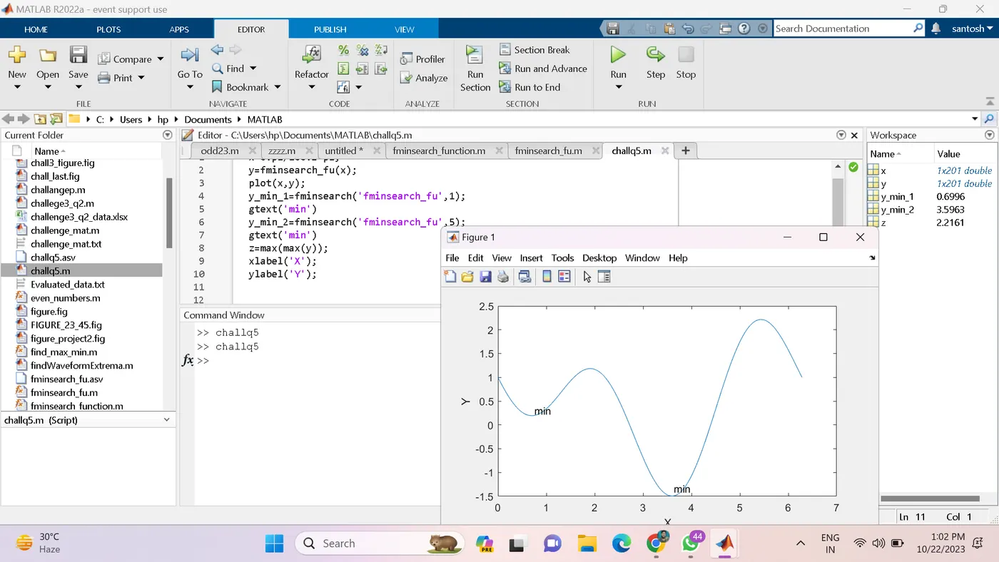
x=0:pi/100:2*pi;
y=fminsearch_fu(x);
plot(x,y);
y_min_1=fminsearch('fminsearch_fu',1);
gtext('min')
y_min_2=fminsearch('fminsearch_fu',5);
gtext('min')
z=max(max(y));
xlabel('X');
ylabel('Y'
PROJECT 4
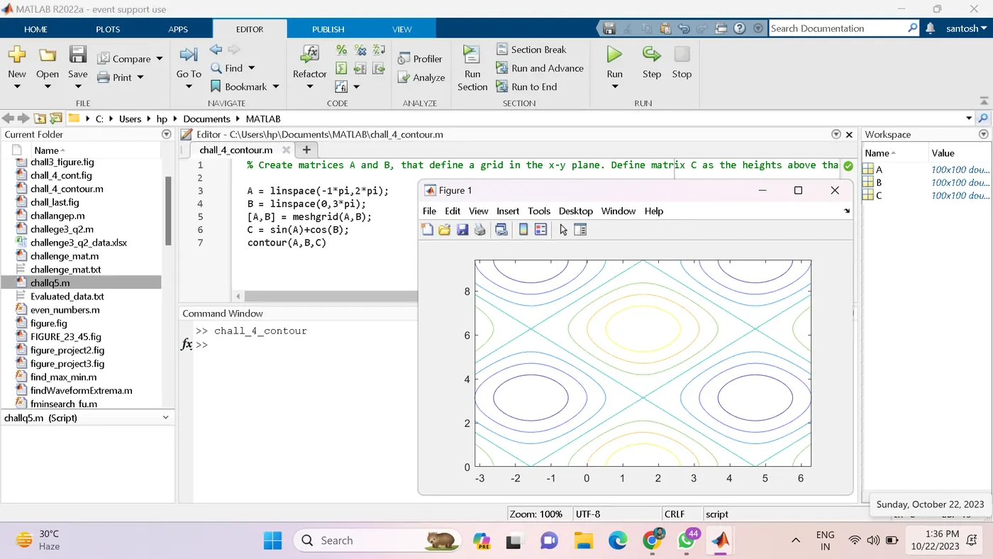
contour Contour plot.
- Contour(Z) draws a contour plot of matrix Z in the x-y plane, with the x-coordinates of the vertices corresponding to column indices of Z and the y-coordinates corresponding to row indices of Z. The contour levels are chosen automatically.
- contour(X,Y,Z) draws a contour plot of Z using vertices from the mesh defined by X and Y. X and Y can be vectors or matrices.
- contour(Z,N) and contour(X,Y,Z,N) draw N contour lines, choosing the levels automatically.
- contour(Z,V) and contour(X,Y,Z,V) draw a contour line for each level specified in vector V. Use contour(Z,[v v]) or ontour(X,Y,Z,[v v]) to draw contours for the single level v.
contour(AX, ...) plots into the axes AX.
- [C,H] = contour(...) returns contour matrix C and a handle, H, to a contour object. These can be used as inputs to CLABEL. The structure of a contour matrix is described in the contour
documentation
EXAMLE :-
% Create matrices A and B, that define a grid in the x-y plane. Define matrix C as the heights above that grid. Then plot the contours of C
A = linspace(-1*pi,2*pi);
B = linspace(0,3*pi);
[A,B] = meshgrid(A,B);
C = sin(A)+cos(B);
contour(A,B,C)