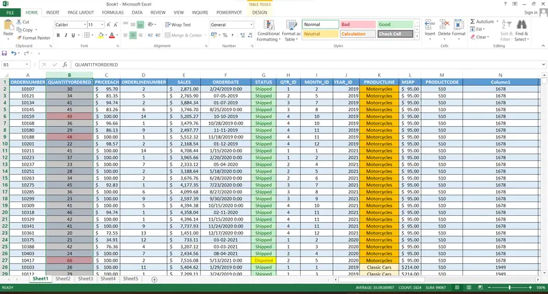
Project 1 - Data Cleaning and Transformation using Pivot table and Charts for the Report on requirement of Team Hiring
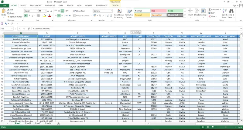
a. Do proper formatting of the data with using borders, font size and appropriate alignment of the content.
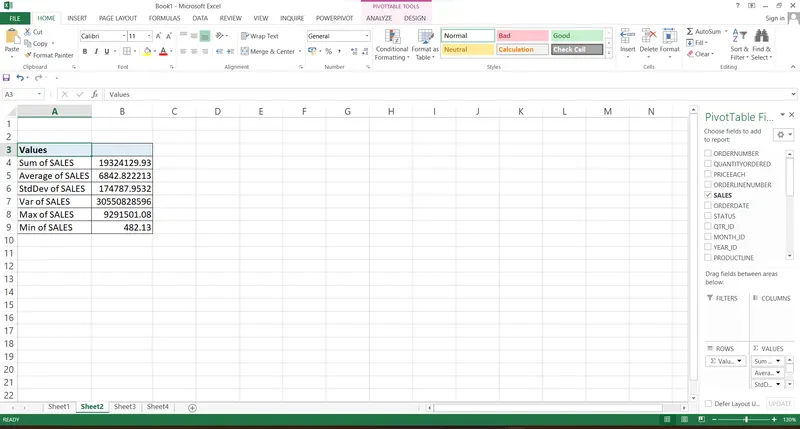
b. Make summary of Products Sales by providing
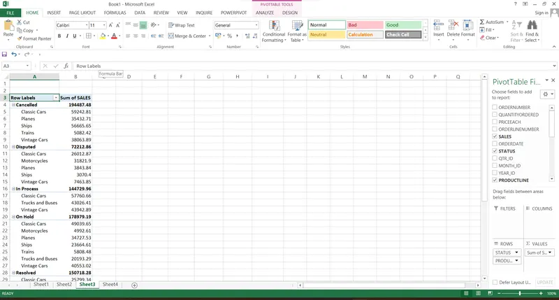
c. Make worksheet from the given Data for categorical representation of table based on fields Status, ProductLine and Sales using Pivot Table.
d. Make Customized Ribbon by naming ABC and keep all data formatting commands in the newly created Ribbon.
Before I show you all the different options you have that you can use to customize the Excel ribbon, let me first show you how to access these options.
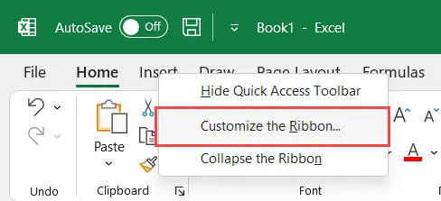
To open the Excel ribbon customization options, right-click on any of the existing tabs in your workbook and then click on the ‘Customize the Ribbon’ option.
This will open the ‘Excel Options’ dialog box, where on the left pane, ‘Customize Ribbon’ option would be selected, and on the right side you would have all the different options available to you.
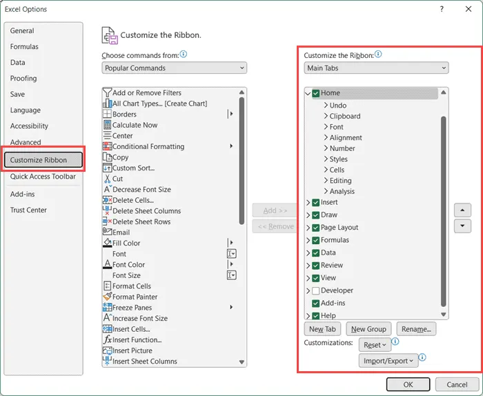
By default, Excel will show you all the tabs in the ribbon, and all the options are available in the selected tab.
For example, below I have the ‘Home’ tab selected and you can also see all the options in the Home tab.

While this is useful, a lot of advanced Excel users do not like that some space on their worksheet is always occupied by these visible options (the ones in each tab), and they would rather have a few extra rows visible rather than see these options.
You can easily collapse (or uncollapse) the Excel ribbon so that you only see the tab names and not the options in the tabs.
To do this, right-click on any of the existing tabs, and then click on the ‘Collapse the Ribbon’ option
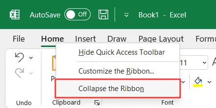
Once the ribbon is collapsed, you would only see the tab names, and the options would only show up when you click on any of the tabs.
And in case you want to get these options back (so that they’re always visible), you can right-click and then click on the ‘Collapse the Ribbon’ option again.
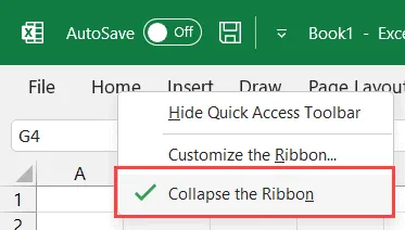
Note that you can also use this option in other Microsoft applications such as MS Word
Rename the Tabs in the Ribbon
While the default tab names are pretty good for me, in case you want to change a tab name, it can easily be done using the below steps:
- Open the Excel Options dialog box (by right-clicking on any of the existing tabs and then clicking on ‘Customize the Ribbon’)
- Right-click on the tab name that you want to rename
- Click on the Rename option
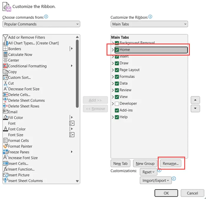
- In the Rename dialog box, enter the name you want to assign to the selected tab
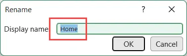
Note that once you change the name of a tab, you won’t be able to revert the change.
In case you want the original tab name back the only way is to either rename the tab again with the original name or reset all the settings for the tab (which also means that you would lose all the customizations that you have done so click here to learn how to reset the customizations done to the tabs.
Create Your Own Group
Options in each tab in the ribbon are further grouped into Groups.
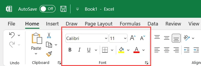
For example in the ‘Home’ tab, we have the ‘Font’ group that has all options related to the font options.
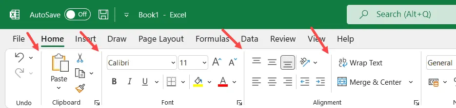
You will notice that these groups are separated from each other by a thin vertical gray line.
While you cannot change the existing groups in a tab in the Robin, you can create your own groups and then add your own commands to each group.
Below are the steps to create your own custom group in an existing tab in the ribbon
- Open the Excel Options dialog box
- Select the tab in which you want to create a custom group. In this example, I will go with the Home tab
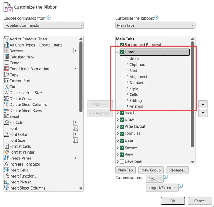
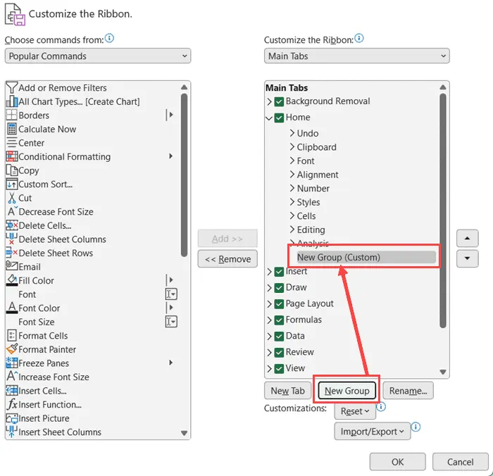
- Click on the New Group option. This will insert a new group with the name ‘New Group (Custom)’
- Add commands to the new group from the list on the left (select the command that you want to add and then click on the add button)
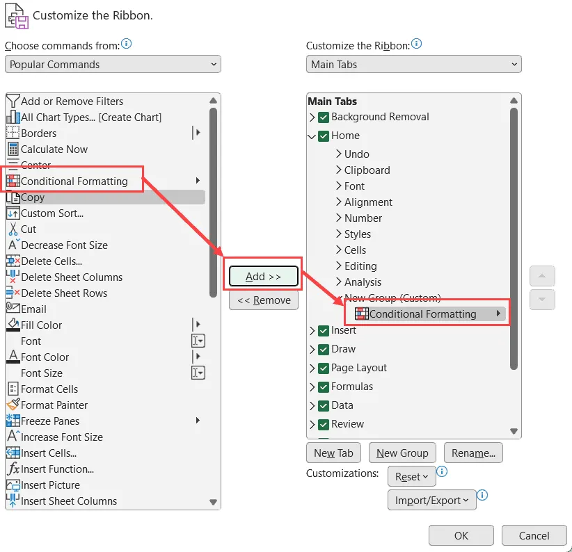
Note that you need to add at least one command to the new custom group that you add, else it would not be reflected in the ribbon when you close the Excel options dialog box.
Below is the screenshot where the new custom group is added to the Home tab.
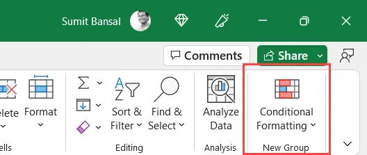
Once you have added the custom group, you can reorder it within the tab by using the up or down arrow key.
To remove the custom group, right-click on it and then click on the Remove option (or select the custom group and then click on the Remove button on the left)
You can also rename the custom group and make it name from meaningful/descriptive
You can also add your own custom tab in the ribbon and then create custom groups and add commands to it.
This could be useful if there are some options that you need to use quite often and would want to have these options together in one tab.
Below are the steps to add your own custom tab in the ribbon in Excel:
- Open the Excel Options dialog box
- Click on the ‘New Tab’ option
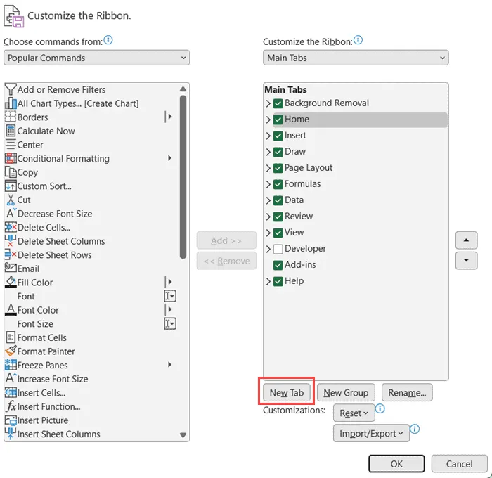
The above steps would insert a new tab in the ribbon with the name ‘New Tab’.
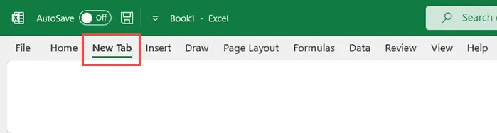
As of now, since we have not added any command in this new tab, it would be blank as of now.
To add commands to this new tab, select the new group option and then add a command from the left by clicking on the Add button.
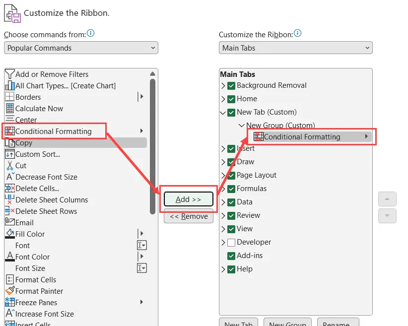
And of course, you can change the name of the new tab as well as all the groups that you insert in this new tab. To change the name, right-click on the New Tab option and then click on Rename.
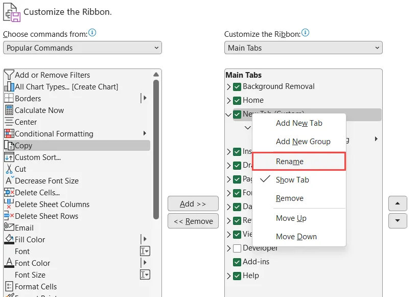
This will open the rename dialog box where you can manually enter the name you want for the new tab.
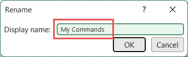
And similarly, to change the name of the new group, right-click on it and then click on rename
How to Add a Command to the Custom Group
When you add a new custom group in any of the tabs in excel, you also need to add a command to that group.
Below are the steps to add a command to a custom group in the Excel ribbon:
- Open the Excel Options dialog box
- Select the group name in which you want to add the command
- Select the command from the list on the left. If you cannot find the command you want to add, you can also show more commands by choosing the ‘All Commands’ option from the ‘Choose command from’ drop-down
- With the command selected, click on the Add button
The above steps would add the selected command to the selected custom group.
And in case you want to remove any command from any of the groups, right-click on it and then click on the remove
Remove Tabs, Groups, and Commands
Excel allows you to remove any of the custom tabs, groups, or commands that you add.
In addition to this, Excel also allows you to remove any of the inbuilt groups in any of the tabs.
However, you cannot remove any of the inbuilt tabs or in-built commands in these tabs.
Below are the steps to remove a group in Excel:
- Open the Excel Options dialog box
- Select the Group that you want to remove
- Click on the ‘Remove’ button (or right-click and then click on Remove)
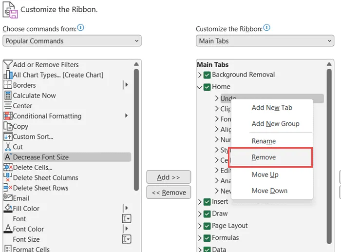
Note that once you remove a group or command, you won’t be able to revert the action. So if you want it back, you would either have to manually add it, or you would have to reset the settings in that tab.
And while you cannot remove the in-built tabs, if you don’t any of the tabs to show up in the ribbon, you can simply uncheck the box before the tab name in the excel options dialog box.
Reset Customizations to get the Default Tab
If you’re customizing the ribbon and he would like to go back to the original default setting, you can easily reset the customizations.
Excel allows you to reset the customizations for specific tabs and the entire ribbon.
Below are the steps to he said the customization for a specific tab (say the Home tab)
- Open the Excel Options dialog box
- Select the Home tab
- Click on the Reset button (which is at the bottom right part of the dialog box)
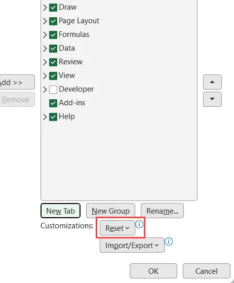
- Click on ‘Reset only selected Ribbon tab’
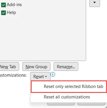
The above steps would reset the selected tab (which is the ‘Home’ tab in this example).
In case there are no customizations done to that tab, the ‘Reset only selected Ribbon tab’ option would be grayed out.
And in case you want to reset the entire ribbon, you can click on the ‘Reset all customizations’ option.
Caution: Once you reset the customizations, you won’t be able to revert them.
Export Your Current Ribbon Customizations
Nowadays, people often use multiple machines for editing the same Excel files. I have my work laptop as well as my travel laptop (a portable Microsoft Surface pro) and I work on both of them on a regular basis.
If I make the ribbon customizations in one of my machines, it would not automatically sync with the other system (given that Excel is a desktop application as of now).
But there’s a better way – you can export all the customizations you have done on one of your systems and then import the file into the other system to apply that customization to the Excel application on that system.
You can also share these customizations with colleagues and other people on your team.
Below are the steps to export the ribbon customizations file in Excel:
- Make all the Ribbon customizations that you want
- Once done, click on the Import/Export button (it’s below the Reset button)
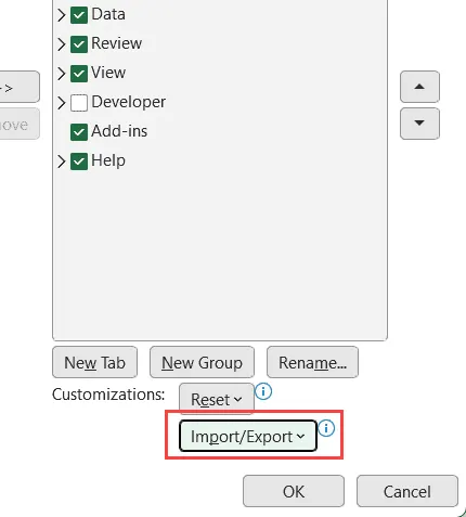
- Click on ‘Export all customizations’
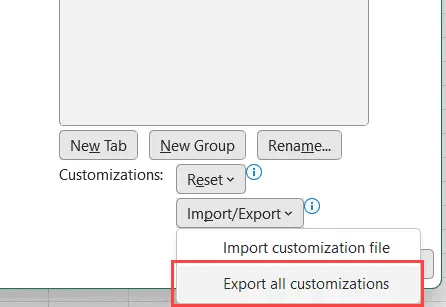
- In the ‘File Save’ dialog box that opens, select the location where you want to save the file.
The above steps would export the customization as a file with the .exportedUI extension.
This file contains all the customizations that you have done, and when you import this file to another system, the same customizations would be applied to it.
Below are the steps to import the customizations:
- Open the Excel Options dialog box
- Click on the ‘Import/Export’ button
- Click on ‘Import customization file’
- In the File Save dialog box that opens, select the file that has the customization
When you import a customization file, remember that you would lose all the customizations that you have done on your Excel application, and the one in the imported file would be application.
e. Analyse the Quantities ordered by each Country in Year 2019,2020 and 2021 for different Quarters using Pivot Table.
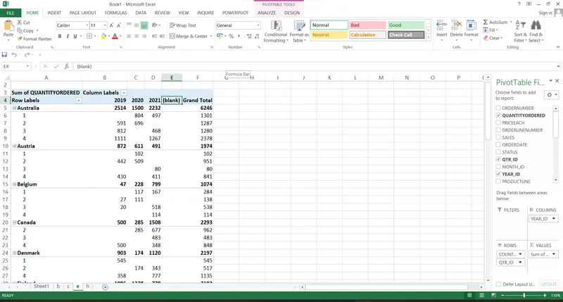
f. Present the data in different colours for values in field Status and ProductLine using conditional formatting.
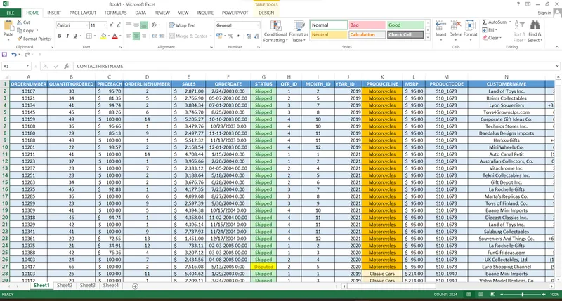
g. Clean the Data with respect to date by proper date formatting and change values of 2003 to 2019, 2004 to 2020 and 2005 to 2021.
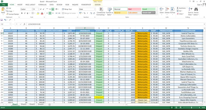
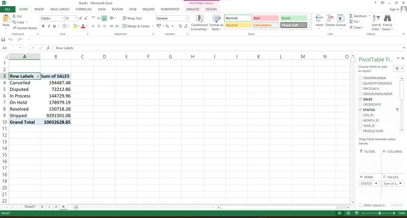
h. Calculate the total sales of all “Shipped”, “Cancelled”, “Disputed”, “In Process”, “On Hold”, “Resolved” products.
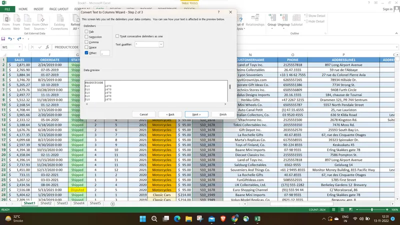
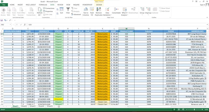
i. Add two new fields in data sheet with reference to Productcode using text functions
Example S10_1678 to S10 _ 1678 .
j. Highlight the top 10% values of QuantityOrdered field using Conditional Formatting